2  Genomic selection of sources

2.1 Setting up

Read in the necessary data for the source optimization. SnpEff v5.1 (Cingolani et al. (2012)) was used to annotate genetic variants to functional class based on Norway spruce genome annotation.

2.1.1 Import annotations from SnpEff

list <- list.files(path = "../../datashare/Spruce/exome_capture/WES_mapping/Annotations/ref_Pglauca/VCF_split_files", 
                   pattern = "Red_Spruce_intersect_poly_", 
                   recursive=TRUE, full.names = T)

# genes <- lapply(list[1], function(x) read.table(x, nrow = 100000)) # originally run for testing
genes <- lapply(list[1], function(x) read.table(x))
category <- lapply(genes, function(x) unlist(lapply(strsplit(as.character(x[,8]), split = "|", fixed = T), function(y) y[2])))

TAB <- genes[1:2]
TAB <- do.call(rbind, TAB)
category <- do.call(c, category)

Read in the meta data for the samples

# Info samples
names <- unlist(lapply(strsplit(unlist(strsplit(as.character(read.table("all_bam.list")[,1]), split = "_rmdup.sorted.bam")), split = "./"), function(x) x[2]))
pops <- unlist(lapply(strsplit(names, split="_"), function(x) x[1]))

info_inds <- read.table("./Info_samples_revised.txt", header=T)
info_inds <- info_inds[match(as.character(names), as.character(info_inds$Family)),]
info_pops <- info_inds[!duplicated(info_inds$Site),-c(1,3,9,10)]

2.1.2 Allele probabilities and frequencies

# Read depth 
depth <- apply(TAB[,-c(1:9)], 2, function(x) as.integer(unlist(lapply(strsplit(as.character(x), split = ":"), function(y) y[2]))))

# Genotype probabilities, changed by NA for the uncovered sites 
gen_prob <- apply(TAB[,-c(1:9)], 2, function(x) unlist(lapply(strsplit(as.character(x), split = ":"), function(y) y[4])))
gen_prob[which(depth==0)] <- NA

# Proba alternative allele
altern_proba <- apply(gen_prob, 2, function(x) (as.numeric(unlist(lapply(strsplit(as.character(x), split = ","), function(y) y[2])))+2*as.numeric(unlist(lapply(strsplit(as.character(x), split = ","), function(z) z[3]))))/2)

# Frequency of the alternative allele for each locus and population
TAB_pop <- lapply(unique(pops),function(x) altern_proba[,which(pops==x)])

names(TAB_pop) <- unique(pops)

freq_pop <- lapply(TAB_pop, function(x) apply(x, 1, function(y) sum(y, na.rm = T)/sum(!is.na(y))))

2.2 Functions to optimize selection

2.2.1 Select regions to select sources

Based on the idea of Regional admixture provenancing (Bucharova et al. (2019)), seed sources were selected regionally for each restoration site. Three groups of source populations were subsetted for the three planting sites, removing XVC and HR because of their northern ancestry. More info on the regional ancestry detailed in Capblancq et al. (2020).

# Sources considered for the Maryland restoration site 
TAB_pop_maryland <- TAB_pop[which(names(TAB_pop)%in%info_pops$Site[which(info_pops$Region=="E" & !info_pops$State%in%c("NC","TN") & !info_pops$Site%in%c("XCV","HR"))])]

# Sources considered for the West Virginia restoration site
TAB_pop_westvirginia <- TAB_pop[which(names(TAB_pop)%in%info_pops$Site[which(info_pops$Region=="E" & info_pops$State=="WV" & !info_pops$Site%in%c("XCV","HR"))])]

# Sources considered for the Virginia restoration site
TAB_pop_virginia <- TAB_pop[which(names(TAB_pop)%in%info_pops$Site[which(info_pops$Region=="E" & (info_pops$State=="WV" & !info_pops$Site%in%c("XCV") | info_pops$Site%in%c("GMF","CR","DG","RP")))])] # remove HR and CV for the paper

2.2.2 Different fucntions applied for source selection

Optimizing genetic diversity

# function to estimate allelic richness after rarefaction
rarefy_AR <- function(data, g, bootstraping=100){
  Nijg <- list()
  Njg <- g*2
  nbind <- ncol(data)
  Nij <- list()
  for(boot in 1:bootstraping){
    inds <- sample(1:nbind, g, replace = FALSE)
    if(g==1){
      Nij[[boot]] <- data[,inds]*2}
    if(g>1){
      Nij[[boot]] <- apply(data[,inds], 1, function(x) sum(x, na.rm = T)/sum(!is.na(x)))*g*2}
  }
  Nijg <- rowMeans(do.call(cbind, Nij), na.rm = T)
  Qijg <- (Njg-Nijg)/Njg
  Pijg <- 1-Qijg
  return(Pijg)
}

Estimate the genetic load

The following function is used to estiamte the ratio of nonsynonymous/synonymous mutation based on the annotation from SnpEff v5.1 (Cingolani et al. (2012)), which was used to annotate genetic variants to functional class based on Norway spruce genome annotation. The functional categories viz. missense variant, splice acceptor variant, splice donor variant, splice region variant, start lost, stop gained, stop lost were used to designate as non-synonymous mutation in our calculation for genetic load.

genetic_load <- function(data, category){
                nonsyn_sites <- which(category=="missense_variant" | category=="splice_acceptor_variant" | category=="splice_donor_variant" | category=="splice_region_variant" | category=="start_lost" | category=="stop_gained" | category=="stop_lost")
                freq_nonsyn <- mean(data[nonsyn_sites], na.rm = T)
                freq_syn <- mean(data[-nonsyn_sites], na.rm = T)
                ratio_2 <- freq_nonsyn/freq_syn
                return(ratio_2)
}

Source selection

This function combines the rarefy_AR and genetic_load function to estimate expected heterozygosity (Hexp), allelic richness and genetic load in all combinations of P populations. The P depends on the number of sources one decides to select for their restoration site.

# function to estimate Hexp, Allelic Richness and Genetic Load in all combination of P populations
optimize <- function(data, P){
  
            # Total diversity and load with all the populations
            TAB_tot <- do.call(cbind,data)
            freq_tot <- apply(TAB_tot, 1, function(y) sum(y, na.rm = T)/sum(!is.na(y)))
            hexp_tot <- mean(2*freq_tot*(1-freq_tot), na.rm = T)
            #all_rich_tot <- mean(rarefy_AR(TAB_tot, ncol(TAB_tot)), na.rm = T)
            genetic_load_tot <- genetic_load(TAB_tot, category)
            
            # Genetic diversity and load with only a subset of P populations
            hexp_sub <- list()
           
            genetic_load_sub <- list()
            names <- list()
            comb <- combn(1:length(data), P, simplify = F)
            for(i in 1:length(comb)){
              TAB_sub <- do.call(cbind, data[comb[[i]]])
              freq_sub <- apply(TAB_sub, 1, function(y) sum(y, na.rm = T)/sum(!is.na(y)))
              hexp_sub[i] <- mean(2*freq_sub*(1-freq_sub), na.rm = T)
              
              genetic_load_sub[i] <- genetic_load(TAB_sub, category)
              names[i] <- paste(names(data[comb[[i]]]), collapse="_")
            }
            TAB_sub <- do.call(rbind, lapply(1:length(hexp_sub), function(x) c(Hexp = hexp_sub[[x]], GenLoad = genetic_load_sub[[x]]))) #AllRich = all_rich_sub[[x]], 
            TAB <- rbind(c(Hexp = hexp_tot, GenLoad = genetic_load_tot), TAB_sub) #AllRich = all_rich_tot, 
            rownames(TAB) <- c("total", unlist(names))
            
            return(TAB)
}

2.2.3 Apply the function to get optimal source combinations

# Optimization sources for site in Maryland
res_maryland <- optimize(TAB_pop_maryland, 3)
which.max(res_maryland[-1,1]/res_maryland[-1,2])
res_maryland[c(1,which.max(res_maryland[-1,1]/res_maryland[-1,2])+1),]

# Optimization sources for site in West Virginia
res_westvirginia_4 <- optimize(TAB_pop_westvirginia, 4)
which.max(res_westvirginia_4[-1,1]/res_westvirginia_4[-1,2])

# Optimization sources for site in Virginia
res_virginia_4 <- optimize(TAB_pop_virginia, 4)
which.max(res_virginia_4[-1,1]/res_virginia_4[-1,2])

2.3 Source list

Even though the optimal source combinations are obtained from the optimize function for each site. Its just a list of recommendations for the restoration practitioners to select from. The final source combination selected depends on the seed availability during the year of procurement.

2.3.1 Plotting with base R

Maryland

## MD
DT::datatable(res_maryland,options = list(pageLength = 5, dom = 'tip'))

hist(res_maryland[,3], xlab="Genetic diversity:Genetic load",main="")


res_maryland["XCS_XDS_XPK",3] 

[1] 0.1808131

abline(v=0.1808131, col="red")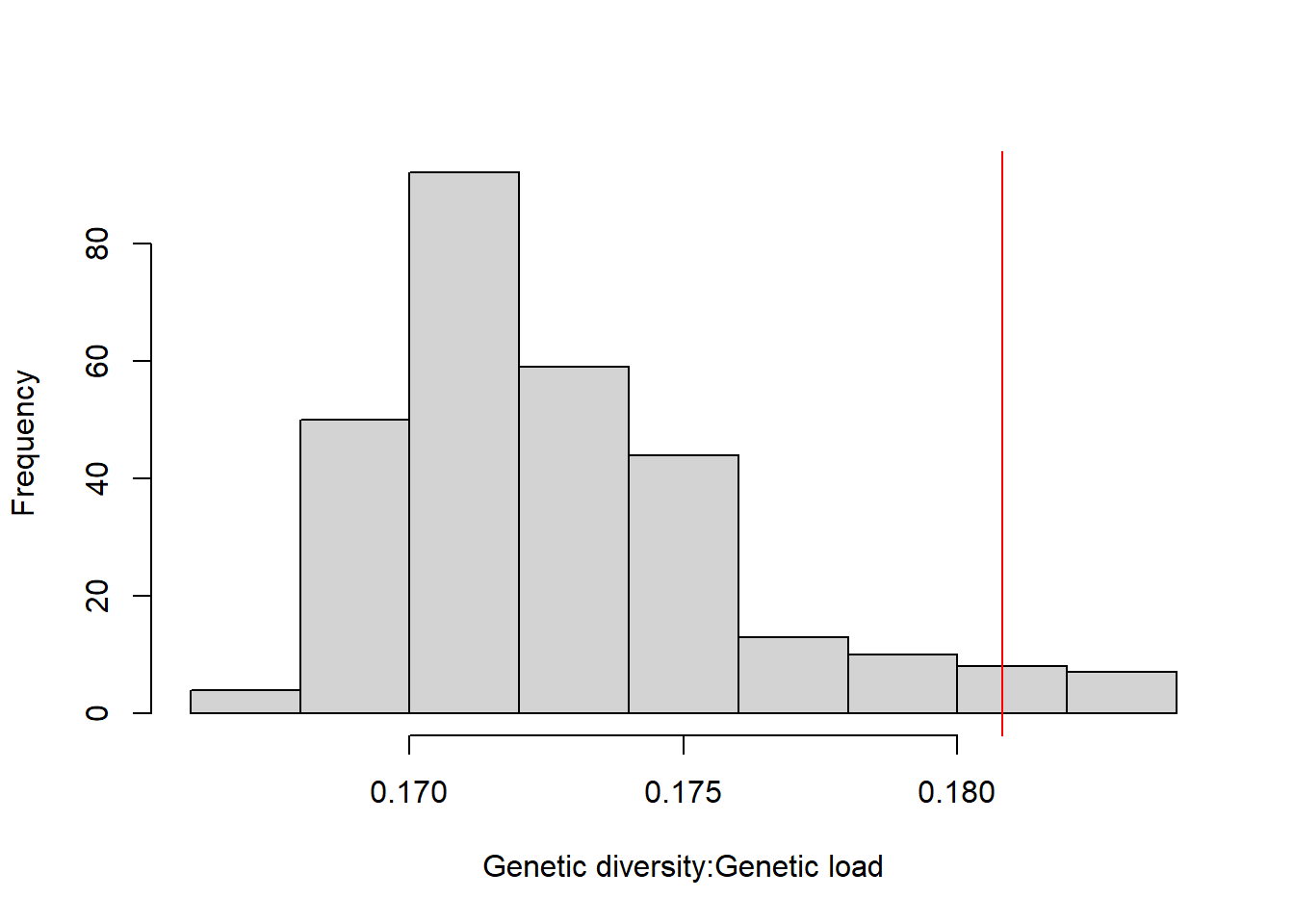

West Virginia

## WV
DT::datatable(res_westvirginia_4,options = list(pageLength = 5, dom = 'tip'))

hist(res_westvirginia_4[,3], xlab="Genetic diversity:Genetic load",main="")
res_westvirginia_4["XCS_XDS_XPK_XSK",3] 

[1] 0.1826622

abline(v=0.1826622, col="red")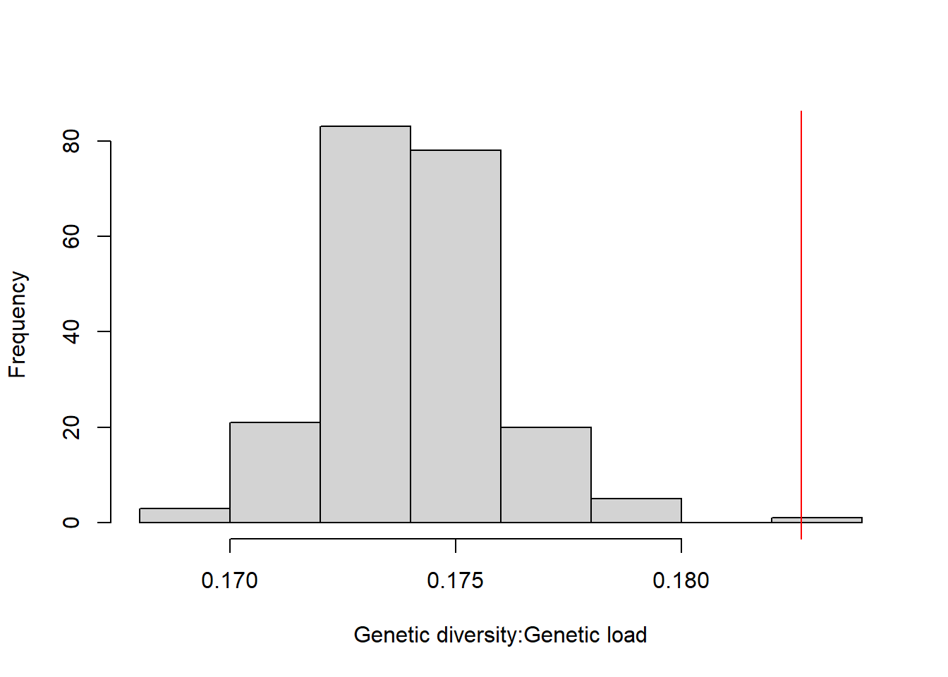

Virginia

## VA
DT::datatable(res_virginia_4,options = list(pageLength = 5, dom = 'tip'))

hist(res_virginia_4[,3], xlab="Genetic diversity:Genetic load",main="")
res_virginia_4["BFA_KOS_XDS_XPK",3] 

[1] 0.1758529

abline(v=0.1758529, col="red")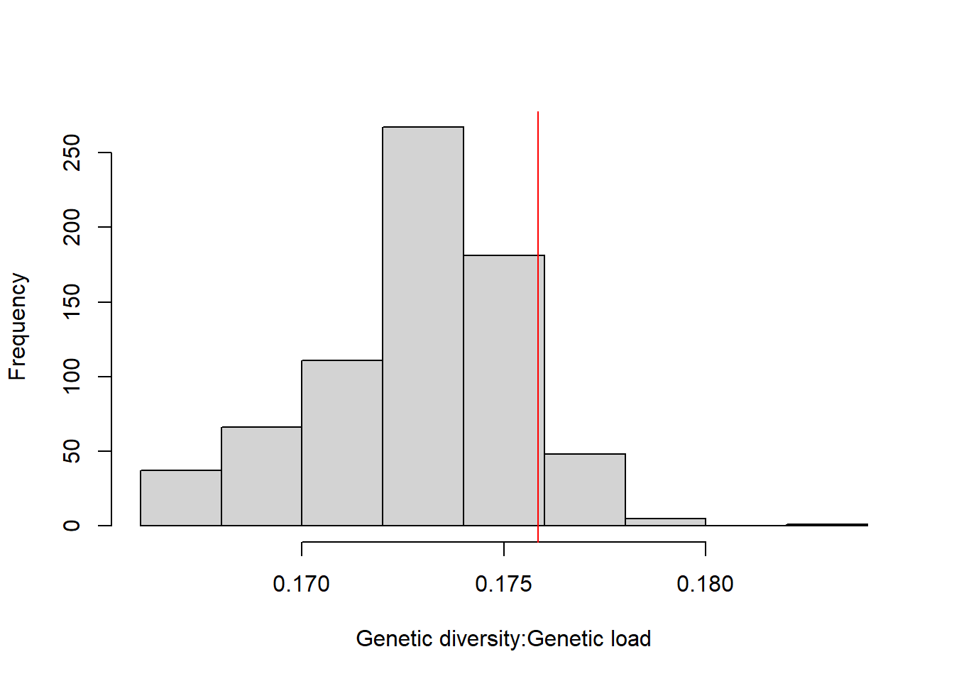

2.3.2 Plotting with ggplot2

Maryland

require(ggplot2)
require(dplyr)
# Maryland final
MD_data <- as.data.frame(res_maryland[,1]/res_maryland[,2])
colnames(MD_data)[1] <- "GD_GL"
MD_data$Sources <- rownames(MD_data)
rownames(MD_data) <- NULL
MD_data <- MD_data[-1,]

MD_plot <-    ggplot(MD_data, aes(x=GD_GL)) +
              geom_histogram(aes(y=..density..),color="#9FE2BF",fill="white", position="dodge", bins=60)+
              geom_density(alpha=.2, fill="#9FE2BF", color="#DFFF00") +
              geom_vline(aes(xintercept=res_maryland["XCS_XDS_XPK",1]/res_maryland["XCS_XDS_XPK",2]),
                         linetype="dashed", color="#7B241C")+
              theme(legend.position="top")

plot1 <- MD_plot + scale_color_brewer(palette="Dark2") +
          theme_minimal()+theme_classic()+theme(legend.position="top") +
          ylab("Frequency") + xlab("Genetic Diversity/Genetic Load") + 
          theme_bw(base_size = 11, base_family = "Times") +
          theme(axis.text=element_text(size=14), 
                axis.title=element_text(size=18),
                panel.background = element_blank(), 
                legend.background = element_blank(), 
                panel.grid = element_blank(), 
                plot.background = element_blank(), 
                legend.text=element_text(size=rel(.8)), 
                strip.text = element_text(size=30),
                legend.position = "none")
plot1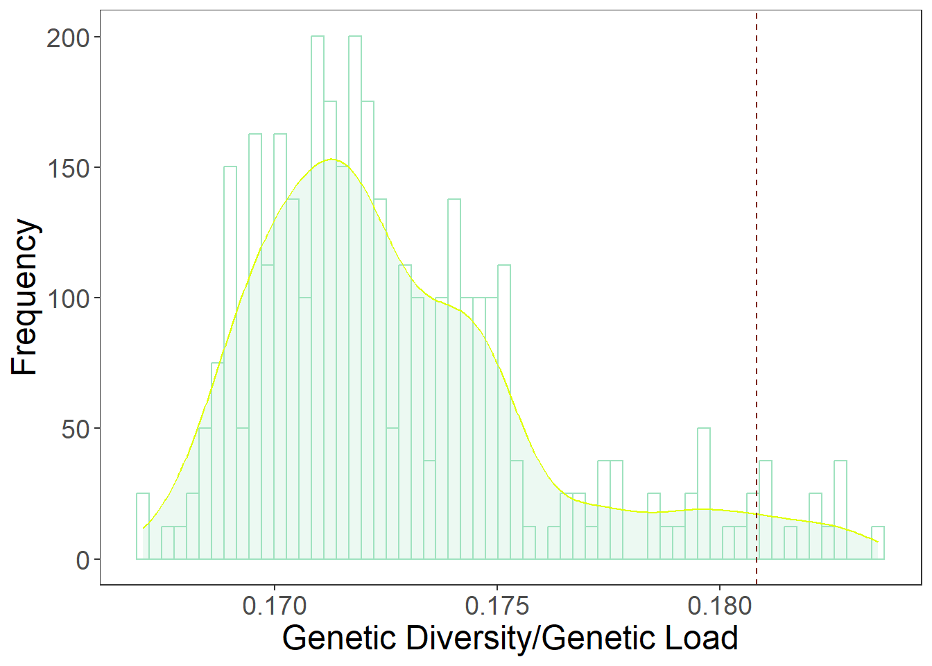

West Virginia

# West Virginia
WV_data <- as.data.frame(res_westvirginia_4[,1]/res_westvirginia_4[,2])
colnames(WV_data)[1] <- "GD_GL"
WV_data$Sources <- rownames(WV_data)
rownames(WV_data) <- NULL
WV_data <- WV_data[-1,]

WV_plot <-    ggplot(WV_data, aes(x=GD_GL)) +
  geom_histogram(aes(y=..density..),color="#FF7F50",fill="white", position="dodge", bins=60)+
  geom_density(alpha=.2, fill="#FF7F50", color="#FFBF00") +
  geom_vline(aes(xintercept=res_westvirginia_4["XCS_XDS_XPK_XSK",1]/res_westvirginia_4["XCS_XDS_XPK_XSK",2]),
             linetype="dashed", color="#7B241C")+
  theme(legend.position="top")

plot2 <- WV_plot + scale_color_brewer(palette="Dark2") +
          theme_minimal()+theme_classic()+theme(legend.position="top") +
          ylab("Frequency") + xlab("Genetic Diversity/Genetic Load") + 
          theme_bw(base_size = 11, base_family = "Times") +
          theme(axis.text=element_text(size=14), 
                axis.title=element_text(size=18),
                panel.background = element_blank(), 
                legend.background = element_blank(), 
                panel.grid = element_blank(), 
                plot.background = element_blank(), 
                legend.text=element_text(size=rel(.8)), 
                strip.text = element_text(size=30),
                legend.position = "none")

plot2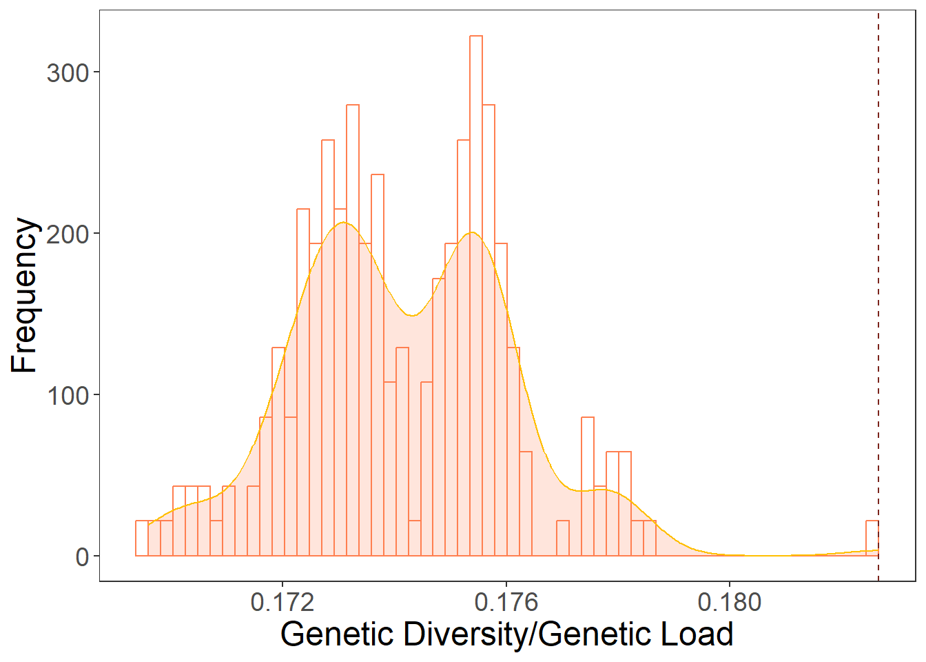

Virginia

# Virginia
VA_data <- as.data.frame(res_virginia_4[,1]/res_virginia_4[,2])
colnames(VA_data)[1] <- "GD_GL"
VA_data$Sources <- rownames(VA_data)
rownames(VA_data) <- NULL
VA_data <- VA_data[-1,]

VA_plot <-    ggplot(VA_data, aes(x=GD_GL)) +
  geom_histogram(aes(y=..density..),color="#CCCCFF",fill="white", position="dodge", bins=60)+
  geom_density(alpha=.2, fill="#CCCCFF", color="#6495ED") +
  geom_vline(aes(xintercept=res_virginia_4["BFA_KOS_XDS_XPK",1]/res_virginia_4["BFA_KOS_XDS_XPK",2]),
             linetype="dashed", color="#7B241C")+
  theme(legend.position="top")

plot3 <- VA_plot + scale_color_brewer(palette="Dark2") +
          theme_minimal()+theme_classic()+theme(legend.position="top") +
          ylab("Frequency") + xlab("Genetic Diversity/Genetic Load") + 
          theme_bw(base_size = 11, base_family = "Times") +
          theme(axis.text=element_text(size=14), 
                axis.title=element_text(size=18),
                panel.background = element_blank(), 
                legend.background = element_blank(), 
                panel.grid = element_blank(), 
                plot.background = element_blank(), 
                legend.text=element_text(size=rel(.8)), 
                strip.text = element_text(size=30),
                legend.position = "none")
plot3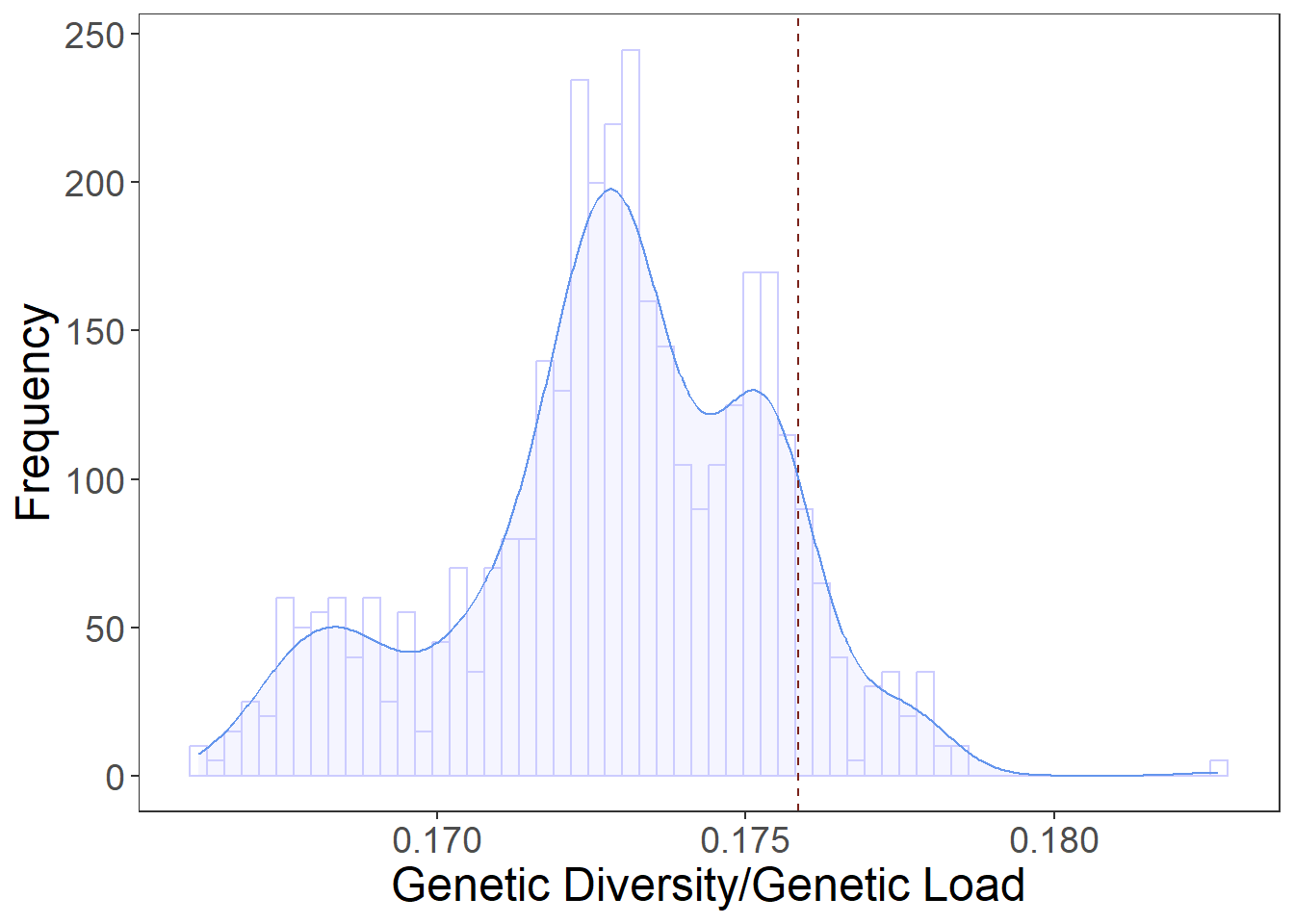

Combine data

# save data for further analysis
MD_reg_GDGL <- as.data.frame(res_maryland)
MD_reg_GDGL$GDGL <- MD_reg_GDGL$Hexp/MD_reg_GDGL$GenLoad

WV_reg_GDGL <- as.data.frame(res_westvirginia_4)
WV_reg_GDGL$GDGL <- WV_reg_GDGL$Hexp/WV_reg_GDGL$GenLoad

VA_reg_GDGL <- as.data.frame(res_virginia_4)
VA_reg_GDGL$GDGL <- VA_reg_GDGL$Hexp/VA_reg_GDGL$GenLoad

GDGL_list <- list()
GDGL_list[[1]] <- MD_reg_GDGL
GDGL_list[[2]] <- WV_reg_GDGL
GDGL_list[[3]] <- VA_reg_GDGL

names(GDGL_list) <- c("Maryland_GDGL","West_Virginia_GDGL","Virginia_GDGL")

# saveRDS(GDGL_list, "./OUTPUT/Genetic_diversity_and_Genetic_load/GDGL_list")

# convert to long data
MD_data2 <- MD_data
MD_data2$Plot <- "Maryland"
WV_data2 <- WV_data
WV_data2$Plot <- "West Virginia"
VA_data2 <- VA_data
VA_data2$Plot <- "Virginia"


GDGL_long_dat <- rbind(MD_data2,WV_data2,VA_data2)
GDGL_long_dat$Plot <- factor(GDGL_long_dat$Plot,levels=c("Maryland","West Virginia","Virginia"))

# figure dim: png(2000h,769w), pdf(7h,18w)
GDGL_plot <- ggplot(GDGL_long_dat, aes(x=GD_GL,color=Plot,fill=Plot)) + facet_wrap(~Plot, scales="free") + 
                # add histogram
                geom_histogram(data=filter(GDGL_long_dat, Plot=="Maryland"), aes(y=..density..),color="#9FE2BF",fill="white", position="dodge", bins=60)+
                geom_histogram(data=filter(GDGL_long_dat, Plot=="West Virginia"), aes(y=..density..),color="#FF7F50",fill="white", position="dodge", bins=60)+
                geom_histogram(data=filter(GDGL_long_dat, Plot=="Virginia"), aes(y=..density..),color="#CCCCFF",fill="white", position="dodge", bins=60)+
                
                # add geom_density
                geom_density(data=filter(GDGL_long_dat, Plot=="Maryland"), alpha=.2, fill="#9FE2BF", color="#40E0D0") + 
                geom_density(data=filter(GDGL_long_dat, Plot=="West Virginia"), alpha=.2, fill="#FF7F50", color="#DE3163") + 
                geom_density(data=filter(GDGL_long_dat, Plot=="Virginia"), alpha=.2, fill="#CCCCFF", color="#6495ED") +
                
                # add vline
                geom_vline(data=filter(GDGL_long_dat, Plot=="Maryland"), 
                           aes(xintercept=res_maryland["XCS_XDS_XPK",1]/res_maryland["XCS_XDS_XPK",2]),
                           linetype="dashed", color="#7B241C") + 
                geom_vline(data=filter(GDGL_long_dat, Plot=="West Virginia"), 
                           aes(xintercept=res_westvirginia_4["XCS_XDS_XPK_XSK",1]/res_westvirginia_4["XCS_XDS_XPK_XSK",2]),
                           linetype="dashed", color="#7B241C") + 
                geom_vline(data=filter(GDGL_long_dat, Plot=="Virginia"), 
                           aes(xintercept=res_virginia_4["BFA_KOS_XDS_XPK",1]/res_virginia_4["BFA_KOS_XDS_XPK",2]),
                           linetype="dashed", color="#7B241C") +
                # theme
                theme_minimal()+theme_classic()+theme(legend.position="top") +
                ylab("Frequency") + xlab("Genetic Diversity/Genetic Load") + 
                theme_bw(base_size = 11, base_family = "Times") +
                theme(axis.text=element_text(size=14), 
                      axis.title=element_text(size=18),
                      panel.background = element_blank(), 
                      legend.background = element_blank(), 
                      panel.grid = element_blank(), 
                      plot.background = element_blank(), 
                      legend.text=element_text(size=rel(.8)), 
                      strip.text = element_text(size=30),
                      legend.position = "none")

Final Viz.

GDGL_plot # check 'Combine data' tab for the plot code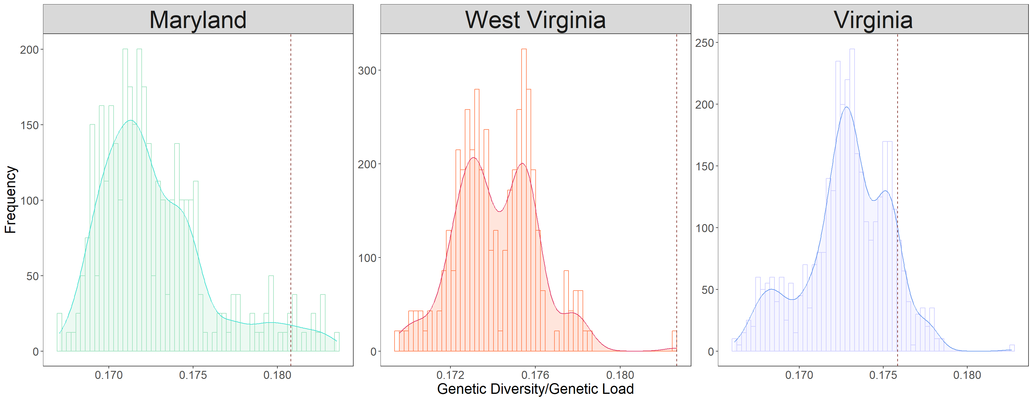

Stats

Maryland

res_maryland <- res_maryland[-1,]
summary(res_maryland)

      Hexp           GenLoad           GDGL       
 Min.   :0.1700   Min.   :0.955   Min.   :0.1671  
 1st Qu.:0.1737   1st Qu.:1.007   1st Qu.:0.1704  
 Median :0.1746   Median :1.015   Median :0.1719  
 Mean   :0.1745   Mean   :1.011   Mean   :0.1727  
 3rd Qu.:0.1755   3rd Qu.:1.020   3rd Qu.:0.1743  
 Max.   :0.1772   Max.   :1.043   Max.   :0.1835  

Which quantile does the selected source GD/GL fall into?

MD_quant <- res_maryland["XCS_XDS_XPK",]$GDGL

# function to estimate which percentile the GD/GL of a source combination falls in
ecdf_fun <- function(x,perc) ecdf(x)(perc)
round(ecdf_fun(res_maryland$GDGL,MD_quant),3)

[1] 0.962

West Virginia

res_westvirginia_4 <- res_westvirginia_4[-1,]
summary(res_westvirginia_4)

      Hexp           GenLoad            GDGL       
 Min.   :0.1747   Min.   :0.9617   Min.   :0.1696  
 1st Qu.:0.1761   1st Qu.:1.0097   1st Qu.:0.1728  
 Median :0.1767   Median :1.0152   Median :0.1739  
 Mean   :0.1767   Mean   :1.0146   Mean   :0.1742  
 3rd Qu.:0.1774   3rd Qu.:1.0191   3rd Qu.:0.1755  
 Max.   :0.1780   Max.   :1.0443   Max.   :0.1827  

Which quantile does the selected source GD/GL fall into?

WV_quant <- res_westvirginia_4["XCS_XDS_XPK_XSK",]$GDGL
round(ecdf_fun(res_westvirginia_4$GDGL,WV_quant),3) 

[1] 1

# best source combination selected based on GD:GL  

Virginia

res_virginia_4 <- res_virginia_4[-1,]
summary(res_virginia_4)

      Hexp           GenLoad            GDGL       
 Min.   :0.1744   Min.   :0.9617   Min.   :0.1661  
 1st Qu.:0.1759   1st Qu.:1.0124   1st Qu.:0.1717  
 Median :0.1764   Median :1.0186   Median :0.1730  
 Mean   :0.1764   Mean   :1.0209   Mean   :0.1729  
 3rd Qu.:0.1770   3rd Qu.:1.0230   3rd Qu.:0.1747  
 Max.   :0.1780   Max.   :1.0527   Max.   :0.1827  

Which quantile does the selected source GD/GL fall into?

VA_quant <- res_virginia_4["BFA_KOS_XDS_XPK",]$GDGL
round(ecdf_fun(res_virginia_4$GDGL,VA_quant),3) 

[1] 0.912

2.4 Saving data for downstream analysis

2.4.1 Creating the GD/GL list

# save data for further analysis
MD_reg_GDGL <- as.data.frame(res_maryland)
MD_reg_GDGL$GDGL <- MD_reg_GDGL$Hexp/MD_reg_GDGL$GenLoad

WV_reg_GDGL <- as.data.frame(res_westvirginia_4)
WV_reg_GDGL$GDGL <- WV_reg_GDGL$Hexp/WV_reg_GDGL$GenLoad

VA_reg_GDGL <- as.data.frame(res_virginia_4)
VA_reg_GDGL$GDGL <- VA_reg_GDGL$Hexp/VA_reg_GDGL$GenLoad

GDGL_list <- list()
GDGL_list[[1]] <- MD_reg_GDGL
GDGL_list[[2]] <- WV_reg_GDGL
GDGL_list[[3]] <- VA_reg_GDGL

names(GDGL_list) <- c("Maryland_GDGL","West_Virginia_GDGL","Virginia_GDGL")

# saveRDS(GDGL_list, "./OUTPUT/Genetic_diversity_and_Genetic_load/GDGL_list")

2.4.2 For source selection maps

MarylandSources <- tail(sort(res_maryland[-1,1]/res_maryland[-1,2]),50)
MarylandSources <- as.data.frame(MarylandSources)
MarylandSources[2] <- rownames(MarylandSources)
rownames(MarylandSources) <- NULL
colnames(MarylandSources)[2] <- "Source_combination"
colnames(MarylandSources)[1] <- "GD/GL"

VirginiaSources <- tail(sort(res_virginia_4[-1,1]/res_virginia_4[-1,2]),50)
VirginiaSources <- as.data.frame(VirginiaSources)
VirginiaSources[2] <- rownames(VirginiaSources)
rownames(VirginiaSources) <- NULL
colnames(VirginiaSources)[2] <- "Source_combination"
colnames(VirginiaSources)[1] <- "GD/GL"


WestVirginiaSources <- tail(sort(res_westvirginia_4[-1,1]/res_westvirginia_4[-1,2]),50)
WestVirginiaSources <- as.data.frame(WestVirginiaSources)
WestVirginiaSources[2] <- rownames(WestVirginiaSources)
rownames(WestVirginiaSources) <- NULL
colnames(WestVirginiaSources)[2] <- "Source_combination"
colnames(WestVirginiaSources)[1] <- "GD/GL"

# write.csv(MarylandSources,"./OUTPUT/MarylandSources_selected_top50.csv")
# write.csv(VirginiaSources,"./OUTPUT/VirginiaSources_selected_top50.csv")
# write.csv(WestVirginiaSources,"./OUTPUT/WestVirginiaSources_selected_top50.csv")

2.4.3 Estimate genetic load and genetic diversity of each pops

# Optimization sources for site in Maryland
res_maryland_singular <- optimize(TAB_pop_maryland, 1)
which.max(res_maryland_singular[-1,1]/res_maryland_singular[-1,2])
res_maryland_singular[c(1,which.max(res_maryland_singular[-1,1]/res_maryland_singular[-1,2])+1),]

# write.csv(res_maryland_singular, "./OUTPUT/Genetic_diversity_and_Genetic_load/maryland_GDGL_per_source")

# Optimization sources for site in West Virginia
res_westvirginia_singular <- optimize(TAB_pop_westvirginia, 1)
which.max(res_westvirginia_singular[-1,1]/res_westvirginia_singular[-1,2])
res_westvirginia_singular[c(1,which.max(res_westvirginia_singular[-1,1]/res_westvirginia_singular[-1,2])+1),]

# write.csv(res_westvirginia_singular, "./OUTPUT/Genetic_diversity_and_Genetic_load/west_virginia_GDGL_per_source")

# Optimization sources for site in Virginia
res_virginia_singular <- optimize(TAB_pop_virginia, 1)
which.max(res_virginia_singular[-1,1]/res_virginia_singular[-1,2])
res_virginia_singular[c(1,which.max(res_virginia_singular[-1,1]/res_virginia_singular[-1,2])+1),]

# write.csv(res_virginia_singular, "./OUTPUT/Genetic_diversity_and_Genetic_load/virginia_GDGL_per_source")

# full sets of pops
TAB_pop_full <- TAB_pop[which(names(TAB_pop)%in%info_pops$Site[which(info_pops$Region=="E" & !info_pops$Site%in%c("XCV","HR"))])]

res_pop_full_singular <- optimize(TAB_pop_full, 1)
which.max(res_pop_full_singular[-1,1]/res_pop_full_singular[-1,2])
res_pop_full_singular[c(1,which.max(res_pop_full_singular[-1,1]/res_pop_full_singular[-1,2])+1),]

Bucharova, Anna, Oliver Bossdorf, Norbert Hölzel, Johannes Kollmann, Rüdiger Prasse, and Walter Durka. 2019. “Mix and Match: Regional Admixture Provenancing Strikes a Balance Among Different Seed-Sourcing Strategies for Ecological Restoration.” Conservation Genetics 20 (1): 7–17. https://doi.org/10.1007/s10592-018-1067-6.

Capblancq, Thibaut, John R. Butnor, Sonia Deyoung, Ethan Thibault, Helena Munson, David M. Nelson, Matthew C. Fitzpatrick, and Stephen R. Keller. 2020. “Whole-Exome Sequencing Reveals a Long-Term Decline in Effective Population Size of Red Spruce (Picea Rubens).” Evolutionary Applications 13 (9): 2190–2205. https://doi.org/10.1111/eva.12985.

Cingolani, Pablo, Adrian Platts, Le Lily Wang, Melissa Coon, Tung Nguyen, Luan Wang, Susan J. Land, Xiangyi Lu, and Douglas M. Ruden. 2012. “A Program for Annotating and Predicting the Effects of Single Nucleotide Polymorphisms, SnpEff: SNPs in the Genome of Drosophila Melanogaster Strain w ¹¹¹⁸ ; Iso-2; Iso-3.” Fly 6 (2): 80–92. https://doi.org/10.4161/fly.19695.