# Simulate one population at one biallelic locus, then summarize it
#   n : number of individuals
#   p : frequency of allele A (0 to 1)
#
# Genotypes are coded 0/1/2:
#   0 = AA, 1 = Aa, 2 = aa
sim_popgen <- function(n, p) {

  q <- 1 - p                       # frequency of allele a

  # 1. Simulate genotypes -------------------------------------------
  #    Under Hardy-Weinberg:  AA = p^2,  Aa = 2pq,  aa = q^2
  genotype <- sample(0:2,
                     size = n,
                     replace = TRUE,
                     prob = c(p^2, 2 * p * q, q^2))

  # 2. Genotype frequencies ----------------------------------------
  geno_freq <- table(genotype) / n

  # 3. Allele frequencies --------------------------------------------
  #    Each genotype value IS an allele-a count, so sum / (2 * n)
  f_a <- sum(genotype) / (2 * n)
  f_A <- 1 - f_a

  # 4. Heterozygosities ---------------------------------------------
  Ho <- sum(genotype == 1) / n      # observed: fraction of Aa
  He <- 2 * f_A * f_a              # expected under H-W: 2pq

  # 5. Print everything -----------------------------------------------
  cat("Allele frequencies:\n")
  cat("  p(A) =", round(f_A, 3), " q(a) =", round(f_a, 3), "\n\n")

  cat("Genotype frequencies:\n")
  print(round(geno_freq, 3))

  cat("\nHeterozygosity:\n")
  cat("  Ho =", round(Ho, 3), " (observed)\n")
  cat("  He =", round(He, 3), " (expected, H-W)\n")

  # Return the results in a list so you can reuse them
  list(genotype = genotype,
       allele_freq = c(A = f_A, a = f_a),
       Ho = Ho,
       He = He)
}R: functions()
hpc
r
foundations
popgen
Writing functions to simply tasks
pop_1 <- sim_popgen(n = 20, p = 0.80) # Population 1 from Part IIAllele frequencies:
p(A) = 0.7 q(a) = 0.3
Genotype frequencies:
genotype
0 1 2
0.5 0.4 0.1
Heterozygosity:
Ho = 0.4 (observed)
He = 0.42 (expected, H-W)pop_2 <- sim_popgen(n = 20, p = 0.30) # Population 2Allele frequencies:
p(A) = 0.275 q(a) = 0.725
Genotype frequencies:
genotype
0 1 2
0.10 0.35 0.55
Heterozygosity:
Ho = 0.35 (observed)
He = 0.399 (expected, H-W)# Combine two populations
pooled <- c(pop_1$genotype, pop_2$genotype)
sum(pooled == 1) / length(pooled) # observed Ho for the pooled data[1] 0.375# Visualize one simulated population against its H-W expectation
plot_popgen <- function(pop, p, n) {
q <- 1 - p
# observed genotype frequencies from the raw genotypes
observed <- table(factor(pop$genotype, levels = 0:2)) / n
# Hardy-Weinberg expectation from the input allele frequency
expected <- c(p^2, 2 * p * q, q^2)
barplot(rbind(observed, expected),
beside = TRUE, # bars side by side, not stacked
col = c("#2A7F8E", "grey75"),
names.arg = c("AA (0)", "Aa (1)", "aa (2)"),
ylab = "frequency",
main = paste0("Observed vs H-W (p = ", p, ")"),
legend = TRUE, bty = "n")
abline(h = 0)
}
plot_popgen(pop_1, p = 0.80, n = 20)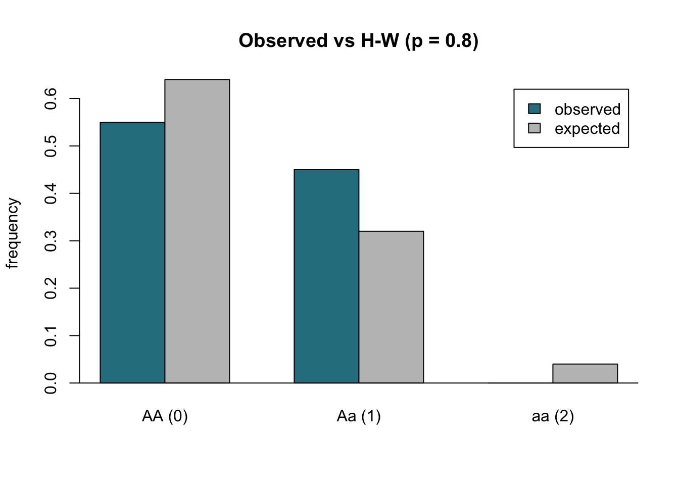
plot_popgen(pop_2, p = 0.30, n = 20)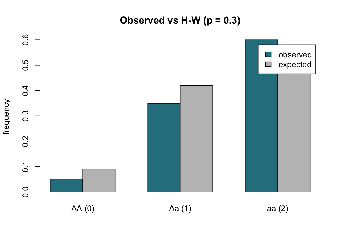
# Pool the raw genotypes and compare against two different expectations
pooled   <- c(pop_1$genotype, pop_2$genotype)
f_a      <- sum(pooled) / (2 * length(pooled))   # pooled allele frequency
f_A      <- 1 - f_a

barplot(rbind(
    "Pooled observed"             = table(factor(pooled, levels = 0:2)) / 40,
    "H-W from pooled p"           = c(f_A^2, 2 * f_A * f_a, f_a^2),
    "Avg of pop expectations"     = (c(0.80^2, 2*.80*.20, 0.20^2) +
                                      c(0.30^2, 2*.30*.70, 0.70^2)) / 2),
    beside    = TRUE,
    col       = c("#583C88", "grey75", "grey50"),
    names.arg = c("AA (0)", "Aa (1)", "aa (2)"),
    ylab      = "frequency",
    main      = "Pooling: the Wahlund effect")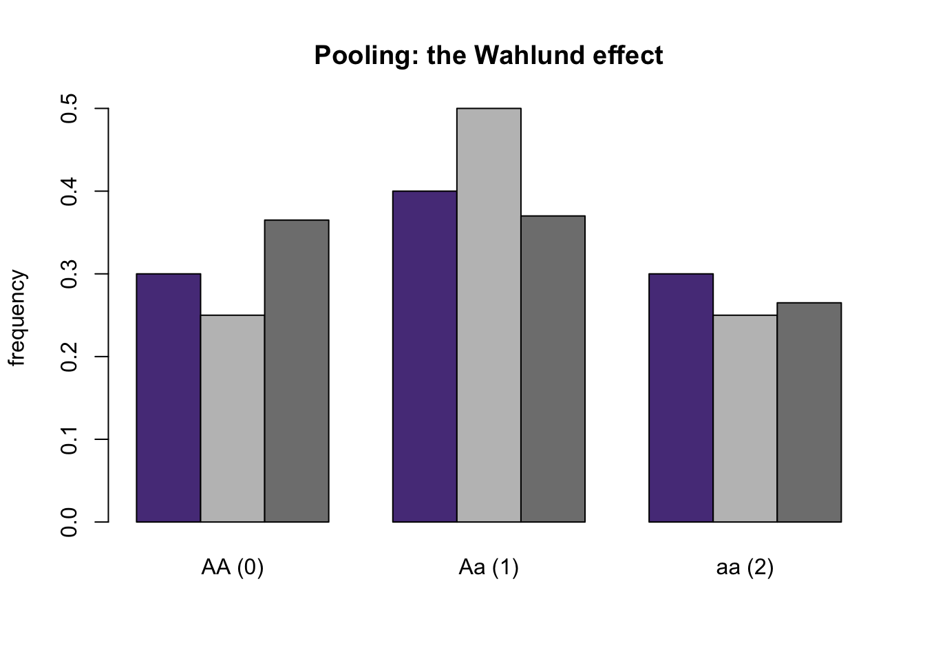
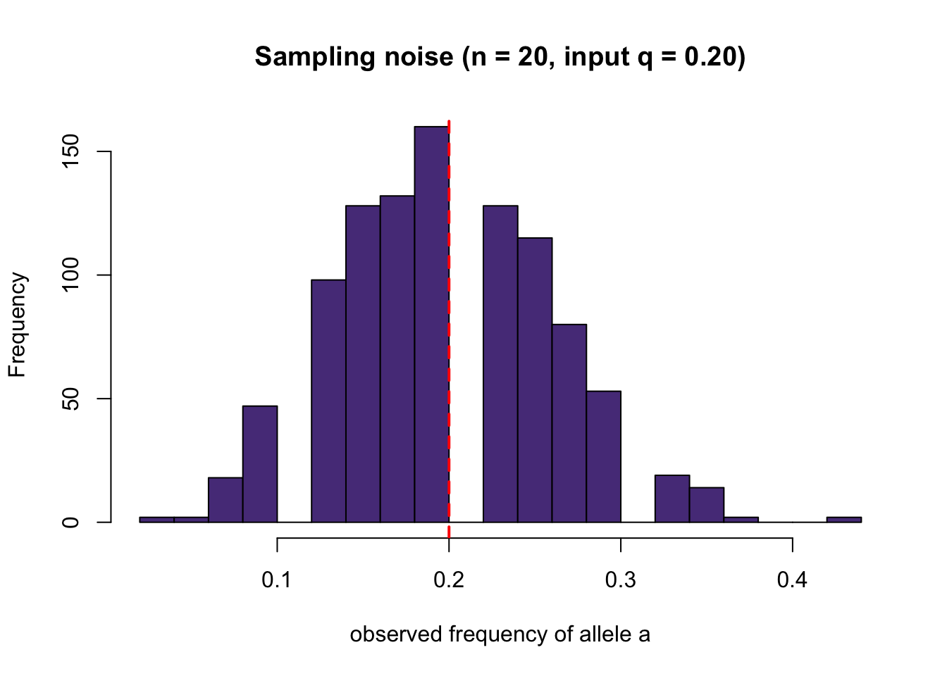
# Run the same simulation 1000 times and collect the observed a frequency
q_obs <- replicate(1000, {
  g <- sample(0:2, 20, replace = TRUE, prob = c(0.80^2, 2*.80*.20, 0.20^2))
  sum(g) / 40
})

hist(q_obs, breaks = 20, col = "#583C88",
     xlab  = "observed frequency of allele a",
     main  = "Sampling noise (n = 20, input q = 0.20)")
abline(v = 0.20, col = "red", lty = 2, lwd = 2)   # the input frequency