
dir.create("data/raw", recursive = TRUE, showWarnings = FALSE)
download.file(
"https://raw.githubusercontent.com/anoobvinu07/Genomic_assisted_selection/master/data/FitnessTraits_GeneticParameters_RedSpruce.txt",
destfile = "data/raw/red_spruce_fitness_traits.txt")R basics for reproducible data analysis
hpc
r
Learn the basics of using R for statistical data analysis
Goal
Learn core R syntax and data-handling skills by analyzing the red-spruce fitness-trait dataset you already downloaded in Bashing the cluster, and finish with a first reproducible R script whose outputs land in results/.
This module picks up exactly where the cluster exercise left off: data/raw/ holds the raw file, src/ will hold your R scripts, and results/ will hold everything R produces.
Prerequisites
- Completed the cluster exercise
- R (>= 4.2) installed; RStudio recommended but not required
- The dataset available at
data/raw/red_spruce_fitness_traits.txt
If you’re working locally instead of on the cluster, grab the same file directly from R:
Recreate the rest of the project layout if you don’t already have it:
dir.create("results", showWarnings = FALSE)
dir.create("src", showWarnings = FALSE)
ImportantProject directory setup
This excercise assumes the project folder follows the following structure:
cluster-exercise/
 ├── data/
 │   └── raw/       # downloaded, unchanged source data
 ├── logs/          # Slurm standard output and error logs
 ├── results/       # analysis products created by R
 └── src/           # R and Slurm scripts
Learning objectives
By the end of this module you should be able to:
- Start R/RStudio with a reproducible working directory (no hard-coded absolute paths)
- Describe R’s core data types and structures: vectors, factors, data frames, lists
- Import and inspect a tab-delimited file
- Subset, filter, and summarize data with base R
- Produce basic plots (histogram, boxplot, scatterplot)
- Save tables and plots into
results/ - Turn interactive code into a script you can run non-interactively with
Rscript
R quick reference
| Function/operator | Purpose | Example |
|---|---|---|
c() |
Combine values into a vector | c(1, 2, 3) |
<- |
Assignment | x <- 5 |
read.delim() |
Read a tab-delimited file | read.delim("data/raw/file.txt") |
str() |
Show structure/types of an object | str(df) |
dim(), nrow(), ncol() |
Dimensions of a data frame | dim(df) |
head() / tail() |
First/last rows | head(df, 5) |
summary() |
Quick numeric/factor summary | summary(df$Height) |
df$col |
Access a column by name | df$Fitness |
df[rows, cols] |
Subset by position/condition | df[df$Region == "E", ] |
table() |
Count occurrences | table(df$Population) |
tapply() / aggregate() |
Grouped summaries | tapply(df$Height, df$Population, mean) |
function(...) {} |
Define a function | f <- function(x) mean(x, na.rm = TRUE) |
for (i in seq) |
Loop | for (p in unique(df$Population)) {...} |
hist(), boxplot(), plot() |
Base R plotting | hist(df$Height) |
write.csv() |
Save a table | write.csv(x, "results/out.csv") |
Setting up your R project
On the cluster, load R and start it from inside cluster-exercise/:
cd ~/projects/cluster-exercise

module biocontainers/default
module load r          # module name may differ on your cluster; check `module avail r`

R                      # start the R session
Inside R, always confirm where you are before reading or writing anything:
getwd()[1] "/Users/anoobprakash/Documents/GitHub/anoobvinu07.github.io/notebook/posts/r-basics"If you’re using RStudio, create an RStudio Project (File > New Project) rooted at cluster-exercise/ — this keeps every path relative and portable, exactly like the data/raw/... paths from the bash module.
R data types and structures
# Vectors: one-dimensional, single type
heights <- c(27.3, 31.1, 29.6, 32.0)
pops    <- c("AB", "AB", "CC", "CC")

# Factors: categorical vectors with fixed levels
region <- factor(c("E", "E", "C", "C"))
levels(region)
[1] "C" "E"# Data frames: a table — columns can be different types
df_demo <- data.frame(pop = pops, height = heights)
str(df_demo)'data.frame': 4 obs. of 2 variables:
$ pop : chr "AB" "AB" "CC" "CC"
$ height: num 27.3 31.1 29.6 32# Lists: can hold mixed, differently-shaped objects
result <- list(mean_height = mean(heights), populations = unique(pops))
result$mean_height[1] 30Key idea: almost everything you do in this module is a data frame — one row per tree, one column per variable — with vectors as its columns.
Importing and inspecting the dataset
traits <- read.delim("data/raw/red_spruce_fitness_traits.txt",
                      header = TRUE, sep = "\t", stringsAsFactors = FALSE)

dim(traits)          # rows x columns
[1] 326 19names(traits) # column names [1] "Family" "Population"
[3] "Tree" "Location"
[5] "Region" "Latitude"
[7] "Longitude" "SeedWeight"
[9] "Germination" "Survival"
[11] "Height" "Fitness"
[13] "Elevation" "PC1"
[15] "PC2" "Family_Homozygosity"
[17] "Population_Homozygosity" "Genetic_Diversity"
[19] "Genetic_Load" str(traits) # types per column'data.frame': 326 obs. of 19 variables:
$ Family : chr "AB_05" "AB_08" "AB_12" "AB_16" ...
$ Population : chr "AB" "AB" "AB" "AB" ...
$ Tree : int 5 8 12 16 1 2 3 5 6 1 ...
$ Location : chr "TN" "TN" "TN" "TN" ...
$ Region : chr "E" "E" "E" "E" ...
$ Latitude : num 35.6 35.6 35.5 35.5 44.3 ...
$ Longitude : num 83.5 83.5 83.5 83.5 70.8 ...
$ SeedWeight : num 0.00387 0.0047 0.00418 0.00348 0.00274 ...
$ Germination : num 0.14 0.04 0.2 0.36 0.78 0.66 0.66 0.72 0.84 0.24 ...
$ Survival : num 0.923 0.692 0.933 0.867 1 ...
$ Height : num 27.3 31.1 29.6 32 23.4 ...
$ Fitness : num 3.531 0.862 5.527 9.976 18.269 ...
$ Elevation : int 1812 1785 1750 1738 455 524 523 573 589 743 ...
$ PC1 : num -0.0446 -0.0395 -0.043 -0.0439 0.0336 ...
$ PC2 : num -0.0569 -0.0747 -0.0598 -0.0606 0.0524 ...
$ Family_Homozygosity : num 0.906 0.888 0.878 0.918 0.89 ...
$ Population_Homozygosity: num 0.0109 0.0109 0.0109 0.0109 0.00684 ...
$ Genetic_Diversity : num 0.0965 0.0965 0.0965 0.0965 0.0945 ...
$ Genetic_Load : num 1.01 1.01 1.01 1.01 1 ...head(traits, 5) # first 5 rows Family Population Tree Location Region Latitude Longitude SeedWeight
1 AB_05 AB 5 TN E 35.55297 83.49438 0.003868
2 AB_08 AB 8 TN E 35.55212 83.49259 0.004702
3 AB_12 AB 12 TN E 35.53890 83.49463 0.004182
4 AB_16 AB 16 TN E 35.53882 83.49534 0.003484
5 ALB_01 ALB 1 ME C 44.30670 70.84019 0.002736
Germination Survival Height Fitness Elevation PC1 PC2
1 0.14 0.9230769 27.32543 3.5312860 1812 -0.04462027 -0.05689514
2 0.04 0.6923077 31.14205 0.8623953 1785 -0.03947036 -0.07471556
3 0.20 0.9333333 29.61083 5.5273541 1750 -0.04297319 -0.05978979
4 0.36 0.8666667 31.97449 9.9760420 1738 -0.04391060 -0.06055466
5 0.78 1.0000000 23.42167 18.2689001 455 0.03360038 0.05241128
Family_Homozygosity Population_Homozygosity Genetic_Diversity Genetic_Load
1 0.9063498 0.010900911 0.09649039 1.014863
2 0.8878673 0.010900911 0.09649039 1.014863
3 0.8783499 0.010900911 0.09649039 1.014863
4 0.9183347 0.010900911 0.09649039 1.014863
5 0.8903996 0.006835856 0.09449166 1.003412summary(traits$Height) Min. 1st Qu. Median Mean 3rd Qu. Max. NA's
19.39 27.04 29.94 30.03 32.38 47.56 13 You should see 19 columns including identifiers (Family, Population, Tree, Location, Region), coordinates and environment (Latitude, Longitude, Elevation), fitness traits (SeedWeight, Germination, Survival, Height, Fitness), and genetic parameters (PC1, PC2, Family_Homozygosity, Population_Homozygosity, Genetic_Diversity, Genetic_Load) — we’ll use that last group in Module 2.
Don’t assume a column’s type from its name — Always check with str() before analyzing.
Indexing and subsetting
# A single column
traits$Fitness |> head() # |> head() : pipe (|>) the additional commands (head()) at the end
[1] 3.5312860 0.8623953 5.5273541 9.9760420 18.2689001 19.9572132# Rows meeting a condition
edge <- traits[traits$Region == "E", ]
nrow(edge)[1] 101# Multiple conditions
healthy_edge <- traits[traits$Region == "E" & traits$Survival > 0.8, ]
# subset() reads more like a sentence
subset(traits, Region == "E" & Height > 35, select = c(Population, Height, Fitness)) Population Height Fitness
83 CRA 37.28518 31.319550
300 XCV 38.33505 21.467628
301 XCV 38.46439 26.155787
326 XWS 35.68774 2.141264Summarizing data
# Counts
table(traits$Population) # number of inds per population
   AB   ALB   APP   ASC     B   BAL   BBE   BER   BFA   BLA   BRA   BRB   BRU
    4     5     6     6     5     6     5     6     5     5     5     4     5
  CAM    CR   CRA   CRR    DG   EQU   ESC   G13   G18   G57   GPA   GRE    HR
    6     5     6     2     5     6     6     5     3    11     4     6     5
  HUN   IND   JAY   KAN   KIL   KOS   LEU   LOL   MAC   MMF   MPG   MRC   MSK
    7     6     3     5     6     6     5     5     5     7     6     5     4
   MT NBTIC   NOR   OCT   OKE   OWL   PRK   PRO    RP   SAV   SPR   TWI    WA
    7     6     6     6     6     4     5     4     5     7     5     5     5
  WCA   WHI   XBM   XCS   XCV   XDS   XFS   XGL   XPK   XSK   XWS
6 6 6 2 5 6 3 4 4 3 3 table(traits$Region) # number of inds per region
  C   E   M
178 101  47
# Grouped means with tapply()
tapply(traits$Height, traits$Population, mean, na.rm = TRUE) AB ALB APP ASC B BAL BBE BER
30.01320 28.57737 29.63241 28.52612 33.56843 35.15642 30.99741 31.03151
BFA BLA BRA BRB BRU CAM CR CRA
28.63783 37.17194 32.56467 25.90857 40.61024 30.87601 28.62938 30.82941
CRR DG EQU ESC G13 G18 G57 GPA
30.85341 26.87212 31.32729 28.55595 27.88004 33.12132 30.55111 29.95064
GRE HR HUN IND JAY KAN KIL KOS
28.31803 29.59271 25.68274 27.40152 25.99047 31.04648 26.37646 28.74159
LEU LOL MAC MMF MPG MRC MSK MT
29.14787 29.32470 27.94443 28.08837 26.60019 27.54005 30.86224 28.95013
NBTIC NOR OCT OKE OWL PRK PRO RP
35.64952 25.63859 31.69911 28.33508 35.86874 29.17456 29.83356 28.79050
SAV SPR TWI WA WCA WHI XBM XCS
31.95079 34.35978 27.82040 26.31308 29.42220 29.29455 38.03620 31.99923
XCV XDS XFS XGL XPK XSK XWS
35.35950 27.99949 25.99399 29.10061 28.37384 26.40402 30.18033 # Grouped summary with aggregate()
aggregate(cbind(Height, Fitness) ~ Population, data = traits, FUN = mean) |> head() Population Height Fitness
1 AB 30.01320 4.974269
2 ALB 28.57737 20.792160
3 APP 29.63241 16.351045
4 ASC 28.52612 18.725993
5 B 33.56843 11.649563
6 BAL 35.15642 14.434015Basic plotting
hist(traits$SeedWeight, main = "Seed weight distribution",
        xlab = "Seed weight")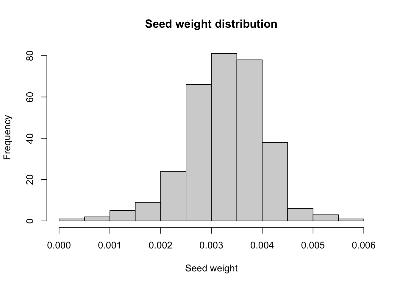
hist(traits$SeedWeight, main = "Seed weight distribution",
        xlab = "Seed weight", breaks = 30)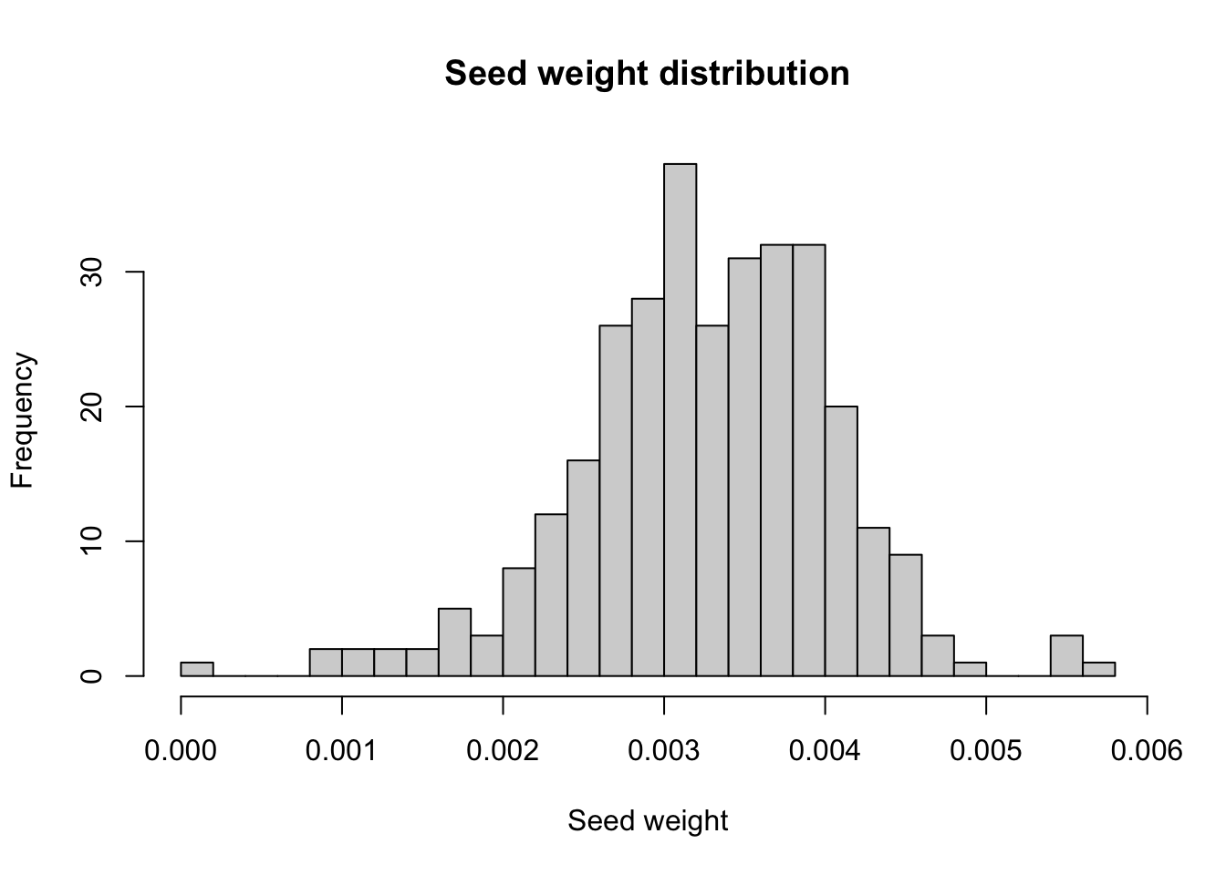
hist(traits$SeedWeight, main = "Seed weight distribution",
        xlab = "Seed weight", breaks = 50)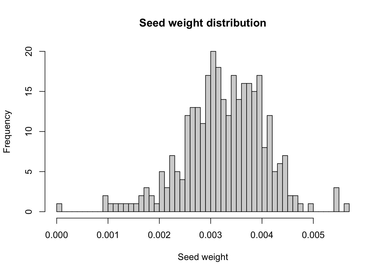
boxplot(Height ~ Region, data = traits,
        main = "Height by region",
        ylab = "Height (cm)")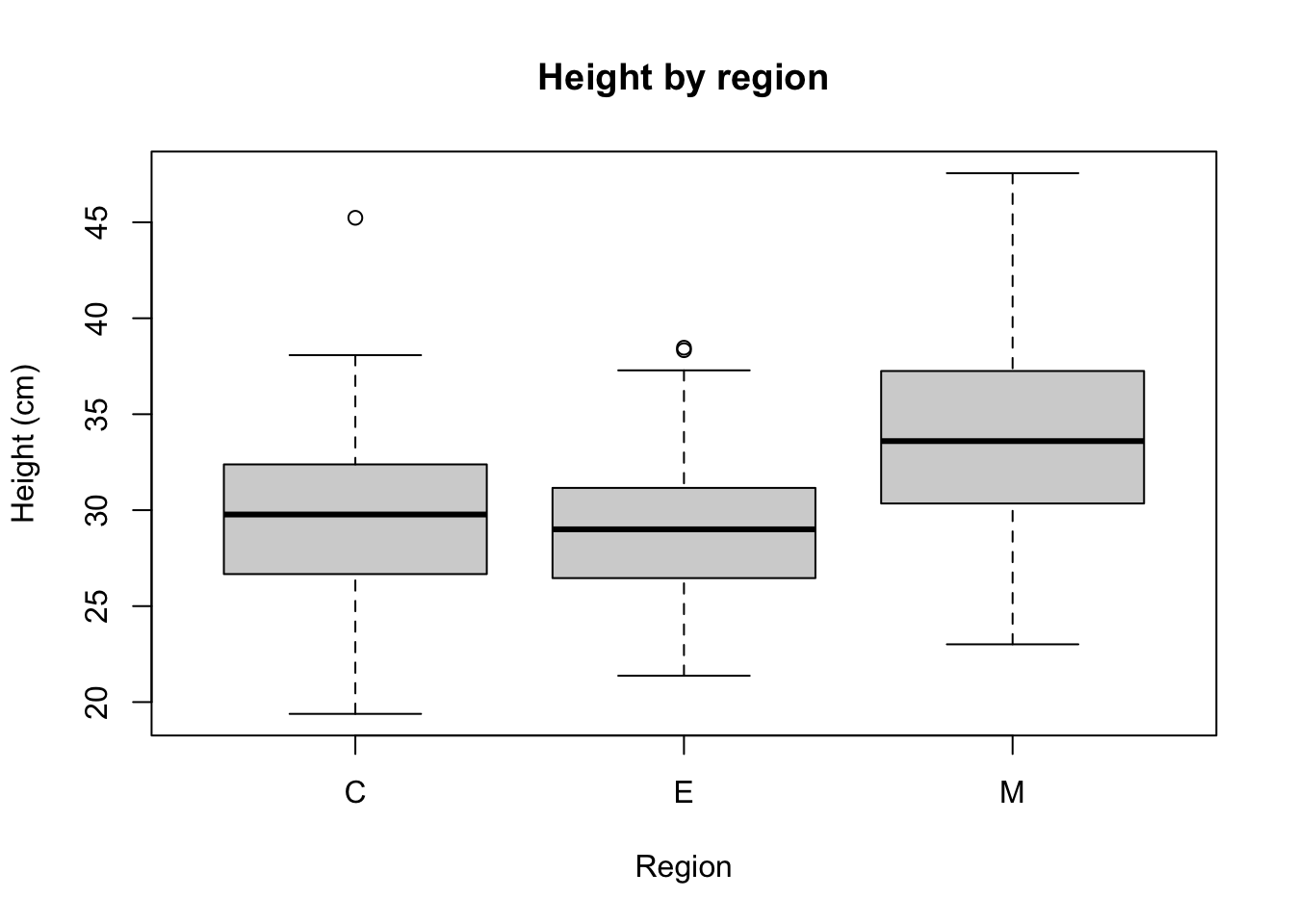
plot(traits$Elevation, traits$Fitness,
     xlab = "Elevation (m)", ylab = "Fitness",
     main = "Fitness vs elevation")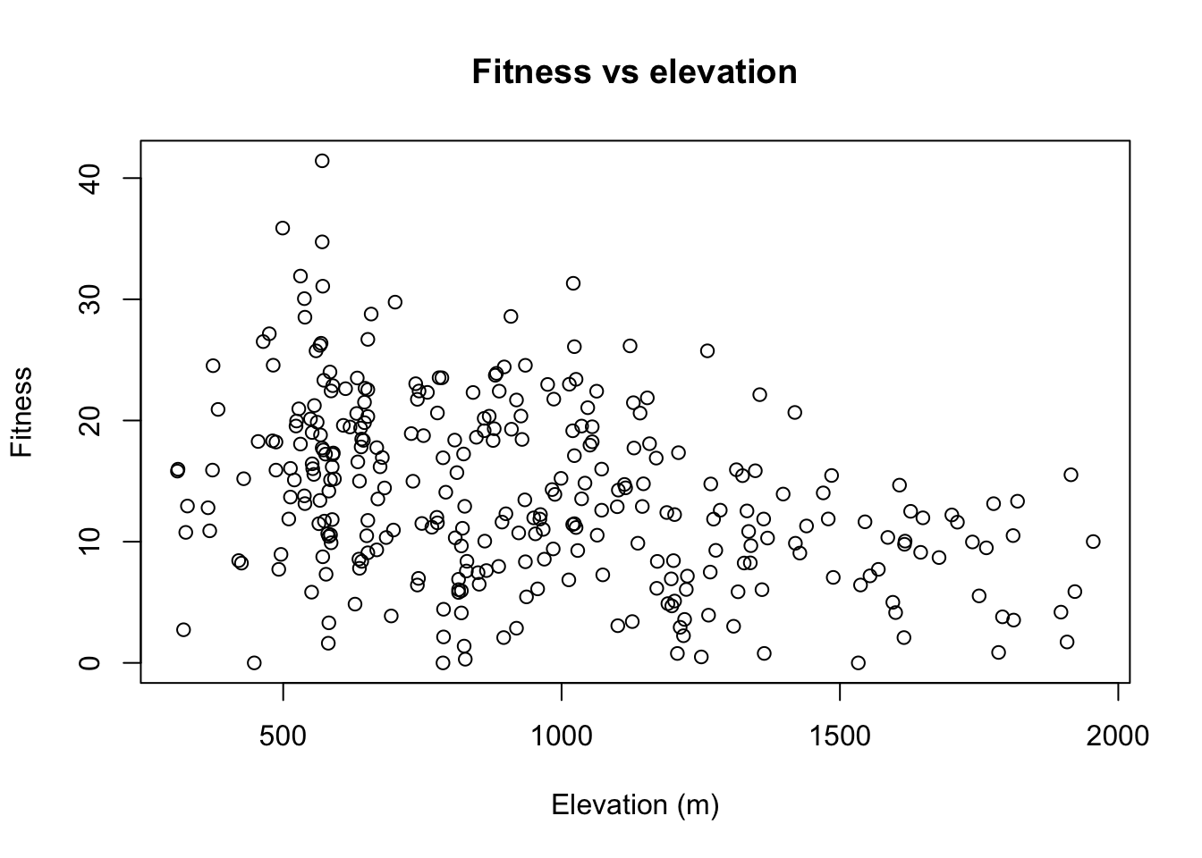
Saving outputs and scripting
pop_summary <- aggregate(cbind(Height, Fitness, SeedWeight) ~ Population, data = traits, FUN = mean)
write.csv(pop_summary, "results/population_trait_summary.csv", row.names = FALSE)
# exporting plot as a .png
png("results/height_by_region.png", width = 800, height = 600)
boxplot(Height ~ Region, data = traits)
dev.off()Put everything into src/01_explore_traits.R and run it non-interactively — this is what makes it reproducible and Slurm-friendly:
Rscript src/01_explore_traits.RWrap up
Idea check
Answer these in your own words before moving to the exercises — write your answers as comments at the top of src/01_explore_traits.R.
- What is the difference between a vector and a data frame in R?
- Why prefer a relative path like
"data/raw/red_spruce_fitness_traits.txt"over an absolute path like/home/your_username/...? - What does
str(traits)tell you thathead(traits)does not? - Why does treating
Regionas afactor(rather than plain character text) matter forboxplot(Height ~ Region, data = traits)? - If
mean(traits$Height)returnedNA, what would you check first, and how would you fix it? - Why write outputs into
results/instead of overwriting anything indata/raw/?
Practical exercises
Work through these in order inside an R session, then consolidate the working code into src/01_explore_traits.R.
- Load the dataset and confirm it has 326 rows and 19 columns.
- Run
str(traits)and list every column name along with its type (chr,int,num). - Compute overall summary statistics (mean, sd, min, max) for
HeightandFitness. - Use
table()to count trees perPopulationand perRegion. Which population has the most trees sampled? - Subset the data to trees in
Region == "C"withSurvival > 0.8. How many trees meet this criterion? - Use
aggregate()ortapply()to get meanHeightand meanFitnessperPopulation. Identify the top 3 populations by meanFitness. - Create a histogram of
SeedWeightand a boxplot ofHeightbyRegion. Save both as PNG files inresults/. - Save your population-level summary table as
results/population_trait_summary.csv. - Move all working code into
src/01_explore_traits.Rand confirm it runs cleanly end-to-end withRscript src/01_explore_traits.R, producing the expected files inresults/.
Homework
- Compute summary statistics (mean, sd, min, max) for at least 4 traits (e.g.,
Height,Fitness,SeedWeight,Germination), broken down by bothPopulationandRegion. - Produce at least 3 plots: one histogram, one boxplot grouped by
Region, and one scatterplot relating two continuous variables (e.g.,Elevationvs.Fitness). Save all three toresults/. - Write your interpretation as comments at the bottom of the script, answering:
- Which population has the highest and lowest mean fitness?
- Is there a visible relationship between elevation and fitness or seed weight? Describe it in one or two sentences.
- Bonus (optional): recreate one plot with
ggplot2instead of base R.