`R`: Module `1` Basics for reproducible data analysis

hpc

Learn the basics of using R for statistical data analysis

Author

Anoob Prakash

Published

September 25, 2026

Modified

October 8, 2026

Goal

Learn core R syntax and data-handling skills by analyzing the red-spruce fitness-trait dataset you already downloaded in Bashing the cluster, and finish with a first reproducible R script whose outputs land in results/.

This module picks up exactly where the cluster exercise left off: data/raw/ holds the raw file, src/ will hold your R scripts, and results/ will hold everything R produces.

Prerequisites

Completed the cluster exercise
R (>= 4.2) installed; RStudio/Positron recommended but not required
The dataset available at data/raw/red_spruce_fitness_traits.txt

If you’re working locally instead of on the cluster, grab the same file directly from R:

# Create directory
dir.create("data/raw", 
recursive = TRUE,      # create the last element of the path- here it will be "raw"
showWarnings = FALSE)


download.file(
"https://raw.githubusercontent.com/anoobvinu07/Genomic_assisted_selection/master/data/FitnessTraits_GeneticParameters_RedSpruce.txt",
      destfile = "data/raw/red_spruce_fitness_traits.txt")

This is work on my system, probably not on yours. Lets use a package called here to make sure that code is reproducibile on your system as well.

# Create directory
dir.create(here::here("data/raw"), 
recursive = TRUE,      # create the last element of the path- here it will be "raw"
showWarnings = FALSE)


download.file(
"https://raw.githubusercontent.com/anoobvinu07/Genomic_assisted_selection/master/data/FitnessTraits_GeneticParameters_RedSpruce.txt",
      destfile = here::here("data/raw/red_spruce_fitness_traits.txt"))

Code reproducibility check

I am using the here package to make this script reproducible. This makes sure that irrespective of of which system this code is run, it will work on that system. Read more about here here.

Instead of calling the package specifically at the top of the script with a library(here) or require(here), I am calling them as a require it. That is done with the syntax packageName::packageFunction. This is useful when you have a lot of packages at the top, but you want to keep track of where a specific function is being called from. There are other reasons as well for following this syntax, for example when you need to call a function that is part of a package not part of the base R. Have you encounetered such situations while coding?

Logic check: what does here::here() actually do?

here::here() answers two questions at once:

Where is the project root? It walks up the directory tree from your working directory until it finds a marker file — a .Rproj file, a .git folder, or a few others. That marker’s directory is the project root.
How do I build a path inside it? Any arguments you pass become folders in order: here::here("data", "raw") returns <project-root>/data/raw with the right separator for your operating system (/ on macOS/Linux, \ on Windows).

Two consequences worth remembering:

The same line, here::here("data/raw/file.txt"), produces the absolute path on your laptop, on the cluster, and on a collaborator’s Windows machine — you never type an absolute path again.
If you open R in the wrong directory (above or beside the project root), here::here() finds no marker and silently falls back to your current working directory — which is why the getwd() / here::here() check below is worth running at the start of every session.

Recreate the rest of the project layout if you don’t already have it:

dir.create(here::here("results"), showWarnings = FALSE)
dir.create(here::here("src"), showWarnings = FALSE)

Note

What is the output when you type in the following commands in your system? What does it mean?

getwd()


here::here()

Answer

getwd() prints your current working directory — the folder R treats as the origin for every relative path you type. If you read.delim("x.txt"), R looks for x.txt there. On the cluster it might be /home/youruser/projects/cluster-exercise; on a laptop, /Users/you/Documents/cluster-exercise.
here::here() called with no arguments prints the project root it detected. On a healthy setup, getwd() and here::here() usually print the same folder — and if they don’t, you’ve opened R somewhere inside the project (say, in src/), and here will still resolve paths correctly while bare relative paths would break. That difference is exactly the bug here prevents.

Project directory setup

This excercise assumes the project folder follows the following structure:

cluster-exercise/
 ├── data/
 │   └── raw/       # downloaded, unchanged source data
 ├── logs/          # Slurm standard output and error logs
 ├── results/       # analysis products created by R
 └── src/           # R and Slurm scripts

Learning objectives

By the end of this module you should be able to:

Start R/RStudio with a reproducible working directory (no hard-coded absolute paths)
Describe R’s core data types and structures: vectors, factors, data frames, lists
Import and inspect a tab-delimited file
Subset, filter, and summarize data with base R
Produce basic plots (histogram, boxplot, scatterplot)
Save tables and plots into results/
Turn interactive code into a script you can run non-interactively with Rscript

R quick reference

Function/operator	Purpose	Example
`c()`	Combine values into a vector	`c(1, 2, 3)`
`<-`	Assignment	`x <- 5`
`class()`	Report the type of an object	`class(traits$Height)`
`is.na()`	Flag missing values	`sum(is.na(traits$Height))`
`na.rm = TRUE`	Skip NAs inside a computation	`mean(x, na.rm = TRUE)`
`read.delim()`	Read a tab-delimited file	`read.delim("data/raw/file.txt")`
`str()`	Show structure/types of an object	`str(df)`
`dim()`, `nrow()`, `ncol()`	Dimensions of a data frame	`dim(df)`
`head()` / `tail()`	First/last rows	`head(df, 5)`
`summary()`	Quick numeric/factor summary	`summary(df$Height)`
`df$col`	Access a column by name	`df$Fitness`
`df[rows, cols]`	Subset by position/condition	`df[df$Region == "E", ]`
`table()`	Count occurrences	`table(df$Population)`
`tapply()` / `aggregate()`	Grouped summaries	`tapply(df$Height, df$Population, mean)`
`function(...) {}`	Define a function	`f <- function(x) mean(x, na.rm = TRUE)`
`for (i in seq)`	Loop	`for (p in unique(df$Population)) {...}`
`hist()`, `boxplot()`, `plot()`	Base R plotting	`hist(df$Height)`
`write.csv()`	Save a table	`write.csv(x, "results/out.csv")`

Setting up your R project

On the cluster, load R and start it from inside cluster-exercise/:


cd ~/projects/cluster-exercise


module biocontainers/default
module load r          # module name may differ on your cluster; check `module avail r`


R                      # start the R session

Inside R, always confirm where you are before reading or writing anything:

getwd()

[1] "/Users/anoobprakash/Documents/GitHub/anoobvinu07.github.io/notebook/learn-to-code/r-basics"

#or


here::here() # when using the here package to set the paths

[1] "/Users/anoobprakash/Documents/GitHub/anoobvinu07.github.io"

If you’re using RStudio, create an RStudio Project (File > New Project) rooted at cluster-exercise/ — this keeps every path relative and portable, exactly like the data/raw/... paths from the bash module.

Logic check: why does the session start matter?

A script that begins by assuming “I am in the right folder” works today and breaks the day you launch R from one directory higher, or copy the project to the cluster. The 10 seconds you spend checking getwd() up front converts a confusing cannot open file 'data/raw/...' error into a one-line fix (setwd() to the right place, or better, restart R in the project root).

Rule of thumb: check the location first, then read files. Every “file not found” error is either a wrong working directory, a typo, or a file that genuinely isn’t there — and the first cause is by far the most common.

R data types and structures

# Vectors: one-dimensional, single type
heights <- c(27.3, 31.1, 29.6, 32.0)
pops    <- c("AB", "AB", "CC", "CC")


# Factors: categorical vectors with fixed levels
region <- factor(c("E", "E", "C", "C"))
levels(region)

[1] "C" "E"

# Data frames: a table — columns can be different types
df_demo <- data.frame(pop = pops, height = heights)
str(df_demo)

'data.frame':   4 obs. of  2 variables:
 $ pop   : chr  "AB" "AB" "CC" "CC"
 $ height: num  27.3 31.1 29.6 32

# Lists: can hold mixed, differently-shaped objects
result <- list(mean_height = mean(heights), populations = unique(pops))
result$mean_height

[1] 30

Key idea: almost everything you do in this module is a data frame — one row per tree, one column per variable — with vectors as its columns.

The four structures, one at a time

A vector is R’s atomic unit: one dimension, one type. Everything you compute with — a column of heights, a column of region labels — is a vector.

heights            # print it

[1] 27.3 31.1 29.6 32.0

class(heights)     # what type is it? "numeric"

[1] "numeric"

length(heights)    # how many elements?

[1] 4

class(pops)        # "character"

[1] "character"

A vector’s type is decided by the most flexible element inside it — this is called implicit coercion, and it is the source of many silent surprises:

c(1, 2, 3)        # numeric: 1 2 3

[1] 1 2 3

c(1, "a")         # character: "1" "a" — the number was demoted to text!

[1] "1" "a"

c(TRUE, 1)        # numeric: 1 1      — TRUE became 1

[1] 1 1

The hierarchy is logical → numeric → character: mixing types in one c() promotes everything to the highest type present. Nothing errors, nothing warns — your 1 just silently becomes "1" and later comparisons like x == 1 stop matching.

A factor is a categorical vector with a fixed, ordered set of levels:

region

[1] E E C C
Levels: C E

as.integer(region)   # stored internally as 2 2 1 1 (E=2, C=1: levels are alphabetical)

[1] 2 2 1 1

table(region)        # counts per level

region
C E 
2 2

Two things make factors different from plain text:

Memory and clarity: a column with 326 "C", "E", "M" strings stores the full text repeatedly; a factor stores small integers plus the level table once.
Fixed classes: levels() defines which categories exist, even if they have zero observations. This matters for counting — as you’ll see with genotypes in population genetics module, table() on a plain vector drops categories that don’t occur, while table(factor(x, levels = ...)) keeps them with a count of zero.

Plotting and modeling functions (boxplot, lm) use levels to decide the order of groups on the axis, which is why the idea check asks about boxplot(Height ~ Region, ...).

A data frame is a list of equal-length vectors displayed as a table — which is why columns can have different types but every column has the same number of rows. It is the structure you will use 95% of the time:

df_demo

  pop height
1  AB   27.3
2  AB   31.1
3  CC   29.6
4  CC   32.0

nrow(df_demo)   # rows = observations

[1] 4

ncol(df_demo)   # columns = variables

[1] 2

One row = one observation (one tree); one column = one variable (its height, its region). This “tidy” layout is what aggregate(), boxplot(Height ~ Region), and almost every R modeling function expect.

A list is a container with no constraints: elements can be different types and different lengths — even other lists. They are how functions bundle multiple outputs:

result

$mean_height
[1] 30

$populations
[1] "AB" "CC"

names(result)    # each slot has a name

[1] "mean_height" "populations"

result$mean_height

[1] 30

You will mostly read lists (model objects, str() output) before you write them, but recognizing [[1]] vs $name access patterns pays off immediately when you start calling summary() on fitted models.

Missing values: `NA`, the silent saboteur

Real datasets have missing data, and this one is no exception — 13 trees are missing a Height measurement. R represents a missing data with NA, and the rule you must internalize is:

Almost any computation that touches an NA returns NA.

x <- c(27.3, 31.1, NA, 32.0)

mean(x)              # NA — R refuses to guess

[1] NA

mean(x, na.rm = TRUE) # 30.13 — "remove NAs, then compute"

[1] 30.13333

is.na(x)              # FALSE FALSE  TRUE FALSE — a logical flag per element

[1] FALSE FALSE  TRUE FALSE

sum(is.na(x))         # 1 — counting NAs by summing TRUEs

[1] 1

sum(!is.na(x))        # 3 — counting non-missing values

[1] 3

Why does sum(is.na(x)) work? is.na() returns a logical vector, and in arithmetic TRUE counts as 1 and FALSE as 0 — so summing counts the TRUEs. That idiom (sum(is.na(col))) is the standard first move when inspecting any new dataset.

NA is contagious in subsetting too — see the indexing section below.

Logic check: predict the output

Before running each line, write down what you expect. Then check.

c(1, 2, 3) > 2

[1] FALSE FALSE  TRUE

mean(c(1, NA, 3))

[1] NA

sum(c(TRUE, TRUE, FALSE))

[1] 2

class(c(TRUE, 2))

[1] "numeric"

table(c("A", "A", "B", NA))


A B 
2 1

Answers

c(1, 2, 3) > 2 → FALSE FALSE TRUE. Comparisons are vectorized: the operation applies element-wise, and the result is a logical vector. This vectorized comparison is the engine behind filtering rows.
mean(c(1, NA, 3)) → NA. No na.rm, no answer. Add na.rm = TRUE to get 2.
sum(c(TRUE, TRUE, FALSE)) → 2. Booleans are 1/0 under arithmetic — the counting trick from the NA section.
class(c(TRUE, 2)) → "numeric". Coercion promotes TRUE to 1, because mixing logical and numeric yields numeric.
table(c("A", "A", "B", NA)) → counts for A (2) and B (1) only, and the NA is silently excluded from the printed table. When checking a dataset, sum(is.na(x)) is more trustworthy than eyeballing table().

Importing and inspecting the dataset

traits <- read.delim(here::here("data/raw/red_spruce_fitness_traits.txt"),
                      header = TRUE, sep = "\t", stringsAsFactors = FALSE)


dim(traits)          # rows x columns

[1] 326  19

names(traits)        # column names

 [1] "Family"                  "Population"             
 [3] "Tree"                    "Location"               
 [5] "Region"                  "Latitude"               
 [7] "Longitude"               "SeedWeight"             
 [9] "Germination"             "Survival"               
[11] "Height"                  "Fitness"                
[13] "Elevation"               "PC1"                    
[15] "PC2"                     "Family_Homozygosity"    
[17] "Population_Homozygosity" "Genetic_Diversity"      
[19] "Genetic_Load"

str(traits)          # types per column

'data.frame':   326 obs. of  19 variables:
 $ Family                 : chr  "AB_05" "AB_08" "AB_12" "AB_16" ...
 $ Population             : chr  "AB" "AB" "AB" "AB" ...
 $ Tree                   : int  5 8 12 16 1 2 3 5 6 1 ...
 $ Location               : chr  "TN" "TN" "TN" "TN" ...
 $ Region                 : chr  "E" "E" "E" "E" ...
 $ Latitude               : num  35.6 35.6 35.5 35.5 44.3 ...
 $ Longitude              : num  83.5 83.5 83.5 83.5 70.8 ...
 $ SeedWeight             : num  0.00387 0.0047 0.00418 0.00348 0.00274 ...
 $ Germination            : num  0.14 0.04 0.2 0.36 0.78 0.66 0.66 0.72 0.84 0.24 ...
 $ Survival               : num  0.923 0.692 0.933 0.867 1 ...
 $ Height                 : num  27.3 31.1 29.6 32 23.4 ...
 $ Fitness                : num  3.531 0.862 5.527 9.976 18.269 ...
 $ Elevation              : int  1812 1785 1750 1738 455 524 523 573 589 743 ...
 $ PC1                    : num  -0.0446 -0.0395 -0.043 -0.0439 0.0336 ...
 $ PC2                    : num  -0.0569 -0.0747 -0.0598 -0.0606 0.0524 ...
 $ Family_Homozygosity    : num  0.906 0.888 0.878 0.918 0.89 ...
 $ Population_Homozygosity: num  0.0109 0.0109 0.0109 0.0109 0.00684 ...
 $ Genetic_Diversity      : num  0.0965 0.0965 0.0965 0.0965 0.0945 ...
 $ Genetic_Load           : num  1.01 1.01 1.01 1.01 1 ...

head(traits, 5)      # first 5 rows

  Family Population Tree Location Region Latitude Longitude SeedWeight
1  AB_05         AB    5       TN      E 35.55297  83.49438   0.003868
2  AB_08         AB    8       TN      E 35.55212  83.49259   0.004702
3  AB_12         AB   12       TN      E 35.53890  83.49463   0.004182
4  AB_16         AB   16       TN      E 35.53882  83.49534   0.003484
5 ALB_01        ALB    1       ME      C 44.30670  70.84019   0.002736
  Germination  Survival   Height    Fitness Elevation         PC1         PC2
1        0.14 0.9230769 27.32543  3.5312860      1812 -0.04462027 -0.05689514
2        0.04 0.6923077 31.14205  0.8623953      1785 -0.03947036 -0.07471556
3        0.20 0.9333333 29.61083  5.5273541      1750 -0.04297319 -0.05978979
4        0.36 0.8666667 31.97449  9.9760420      1738 -0.04391060 -0.06055466
5        0.78 1.0000000 23.42167 18.2689001       455  0.03360038  0.05241128
  Family_Homozygosity Population_Homozygosity Genetic_Diversity Genetic_Load
1           0.9063498             0.010900911        0.09649039     1.014863
2           0.8878673             0.010900911        0.09649039     1.014863
3           0.8783499             0.010900911        0.09649039     1.014863
4           0.9183347             0.010900911        0.09649039     1.014863
5           0.8903996             0.006835856        0.09449166     1.003412

summary(traits$Height)

   Min. 1st Qu.  Median    Mean 3rd Qu.    Max.    NA's 
  19.39   27.04   29.94   30.03   32.38   47.56      13

You should see 19 columns including identifiers (Family, Population, Tree, Location, Region), coordinates and environment (Latitude, Longitude, Elevation), fitness traits (SeedWeight, Germination, Survival, Height, Fitness), and genetic parameters (PC1, PC2, Family_Homozygosity, Population_Homozygosity, Genetic_Diversity, Genetic_Load) — we’ll use that last group in the Population genetics foundation module.

Don’t assume a column’s type from its name — Always check with str() before analyzing.

Code breakdown: what each inspection function told you

dim(traits) → 326 19: 326 rows (trees) and 19 columns (variables). Confirm the row count matches your expectation from the raw file — a mismatch usually means a wrong sep or header argument.
names(traits) → the 19 column names. You will type these constantly; check spelling here first when object not found errors appear later.
str(traits) → the full type map: identifiers are chr (text), Tree and Elevation are int (integers), everything numeric with decimals is num. The three-letter prefixes mean: chr = character, int = integer, num = numeric (double). int columns are numeric for computation — the distinction only matters for storage and factor conversion.
head(traits, 5) → the first 5 rows as they sit in the file — useful for spotting parsing disasters (values in the wrong column, text where numbers should be).
summary(traits$Height) → Min 19.39, Median 29.94, Mean 30.03, Max 47.56 — and 13 NAs. The dataset genuinely has 13 trees with no height measurement. This single line is why the NA section above exists: without na.rm = TRUE, every mean, sd, and correlation on this column is NA.

Worked example: reading a new file safely

The routine to run on any new tabular file, before you analyze anything:

# 1. How big is it? Does the shape match the source?
dim(traits)

# 2. What are the columns called, and what type did R guess?
str(traits)

# 3. Does the first rows look like the actual file (compare to the raw text)?
head(traits)

# 4. Where are the holes?
colSums(is.na(traits))

# 5. Do the categorical columns have the levels I expect?
table(traits$Region)

For this dataset step 4 reports: SeedWeight 12, Germination 12, Survival 1, Height 13, Fitness 12, Elevation 3 — everything else is complete. Knowing this before computing anything is what separates a smooth analysis from an hour of “why is my mean NA?”

Indexing and subsetting

# A single column
traits$Fitness |> head() # |> is called the pipe command, which lets you run the additional commands (head()) at the end

[1]  3.5312860  0.8623953  5.5273541  9.9760420 18.2689001 19.9572132

# Rows meeting a condition
edge <- traits[traits$Region == "E", ]
nrow(edge)

[1] 101

# Multiple conditions
healthy_edge <- traits[traits$Region == "E" & traits$Survival > 0.8, ]


# subset() reads more like a sentence
subset(traits, Region == "E" & Height > 35, select = c(Population, Height, Fitness))

    Population   Height   Fitness
83         CRA 37.28518 31.319550
300        XCV 38.33505 21.467628
301        XCV 38.46439 26.155787
326        XWS 35.68774  2.141264

How the bracket syntax works

df[rows, cols] — the comma splits rows from columns, and an empty slot means “everything”:

Code	Meaning
`df[1, ]`	row 1, all columns
`df[, 2]`	all rows, column 2
`df[1:5, c("Height", "Fitness")]`	rows 1–5, two named columns
`df[df$Region == "E", ]`	every row where the condition is TRUE, all columns
`df[, -1]`	all rows, drop column 1

The filter df[condition, ] works because the condition is a logical vector with one TRUE/FALSE per row, and bracket-indexing keeps exactly the rows whose position is TRUE. That is the vectorized comparison from the logic check, doing real work.

Three beginner traps:

== vs =. == compares (“is Region equal to E?”); = assigns or names arguments. traits[traits$Region = "E", ] is a syntax error.
& vs |. & is AND (both conditions), | is OR (either). For filter vectors use the single forms — &&/|| only compare single values.
NA rows vanish. The one tree with missing Survival makes traits$Survival > 0.8 evaluate to NA for that row, and [ drops NA rows silently. Usually harmless (that row can’t satisfy the condition anyway) — but if you need to keep or count them explicitly, use which() or complete.cases():

# Explicit about missing data: keep only rows with no NA anywhere
traits_complete <- traits[complete.cases(traits), ]
nrow(traits_complete)   # rows surviving the NA filter

[1] 309

Logic check: what did the subsetting code return?

edge keeps 101 rows — the number of trees from Region “E”. Nothing about the filter changed column count: ncol(edge) is still 19.
healthy_edge applies two conditions at once with &; only rows that are Region “E” and have Survival above 0.8 survive.
subset(..., select = c(...)) does both jobs in one call: filter rows and pick columns — its output has only 3 columns. Note it’s a convenient interactive shortcut; the bracket syntax is what scripts and functions reliably use.

Summarizing data

# Counts
table(traits$Population) # number of inds per population


   AB   ALB   APP   ASC     B   BAL   BBE   BER   BFA   BLA   BRA   BRB   BRU 
    4     5     6     6     5     6     5     6     5     5     5     4     5 
  CAM    CR   CRA   CRR    DG   EQU   ESC   G13   G18   G57   GPA   GRE    HR 
    6     5     6     2     5     6     6     5     3    11     4     6     5 
  HUN   IND   JAY   KAN   KIL   KOS   LEU   LOL   MAC   MMF   MPG   MRC   MSK 
    7     6     3     5     6     6     5     5     5     7     6     5     4 
   MT NBTIC   NOR   OCT   OKE   OWL   PRK   PRO    RP   SAV   SPR   TWI    WA 
    7     6     6     6     6     4     5     4     5     7     5     5     5 
  WCA   WHI   XBM   XCS   XCV   XDS   XFS   XGL   XPK   XSK   XWS 
    6     6     6     2     5     6     3     4     4     3     3

table(traits$Region)     # number of inds per region


  C   E   M 
178 101  47

# Grouped means with tapply()
tapply(traits$Height, traits$Population, mean, na.rm = TRUE)

      AB      ALB      APP      ASC        B      BAL      BBE      BER 
30.01320 28.57737 29.63241 28.52612 33.56843 35.15642 30.99741 31.03151 
     BFA      BLA      BRA      BRB      BRU      CAM       CR      CRA 
28.63783 37.17194 32.56467 25.90857 40.61024 30.87601 28.62938 30.82941 
     CRR       DG      EQU      ESC      G13      G18      G57      GPA 
30.85341 26.87212 31.32729 28.55595 27.88004 33.12132 30.55111 29.95064 
     GRE       HR      HUN      IND      JAY      KAN      KIL      KOS 
28.31803 29.59271 25.68274 27.40152 25.99047 31.04648 26.37646 28.74159 
     LEU      LOL      MAC      MMF      MPG      MRC      MSK       MT 
29.14787 29.32470 27.94443 28.08837 26.60019 27.54005 30.86224 28.95013 
   NBTIC      NOR      OCT      OKE      OWL      PRK      PRO       RP 
35.64952 25.63859 31.69911 28.33508 35.86874 29.17456 29.83356 28.79050 
     SAV      SPR      TWI       WA      WCA      WHI      XBM      XCS 
31.95079 34.35978 27.82040 26.31308 29.42220 29.29455 38.03620 31.99923 
     XCV      XDS      XFS      XGL      XPK      XSK      XWS 
35.35950 27.99949 25.99399 29.10061 28.37384 26.40402 30.18033

# Grouped summary with aggregate()
aggregate(cbind(Height, Fitness) ~ Population, data = traits, FUN = mean) |> head()

  Population   Height   Fitness
1         AB 30.01320  4.974269
2        ALB 28.57737 20.792160
3        APP 29.63241 16.351045
4        ASC 28.52612 18.725993
5          B 33.56843 11.649563
6        BAL 35.15642 14.434015

What each summarizer is for

Function	Question it answers	Key arguments
`table()`	How many observations per category?	the categorical vector
`tapply()`	Apply one function to one column, split by one group	(values, groups, function)
`aggregate()`	Same, but multiple columns and multiple groups at once	formula like `cbind(a, b) ~ group`

The formula syntax (Height ~ Population) reads right-to-left: “height, explained by population” — split Height by Population. cbind() glues several response columns together so one call summarizes all of them.

Notice the na.rm = TRUE inside tapply(): it is passed through to mean(). Without it, every population containing one of the 13 missing heights would report NA — and with this dataset, that would be most of them. When a grouped summary comes back full of NAs, this is the first thing to check.

# The formula version of aggregate with two grouping factors
aggregate(Height ~ Region, data = traits, FUN = mean)

  Region   Height
1      C 29.68908
2      E 28.88793
3      M 34.03509

Basic plotting

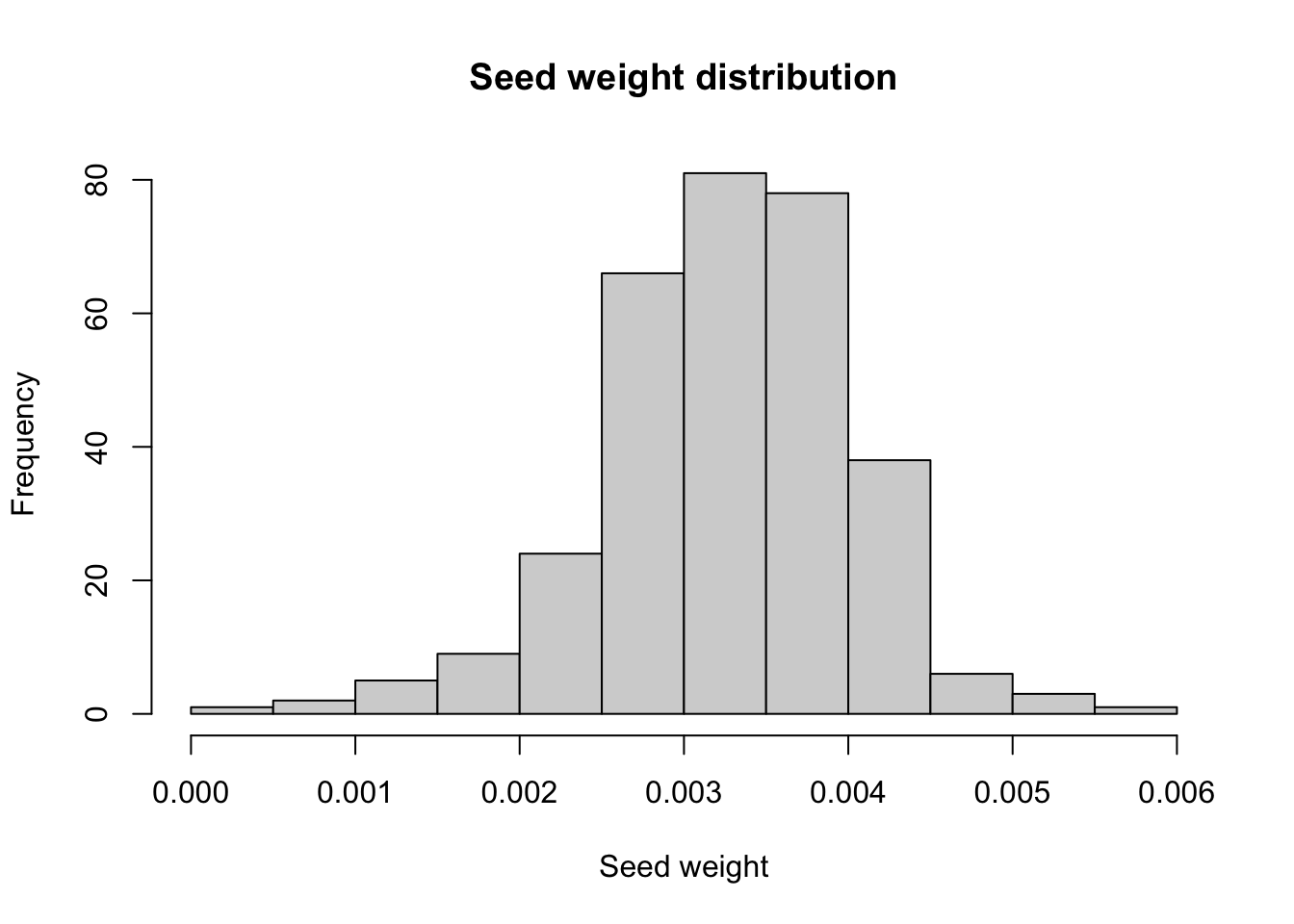
hist(traits$SeedWeight, main = "Seed weight distribution", 
        xlab = "Seed weight")

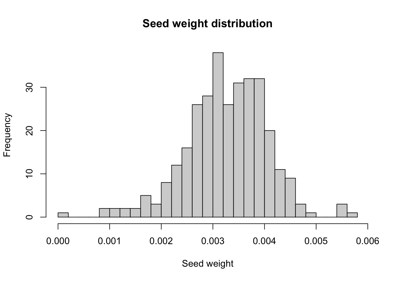
hist(traits$SeedWeight, main = "Seed weight distribution", 
        xlab = "Seed weight", breaks = 30)

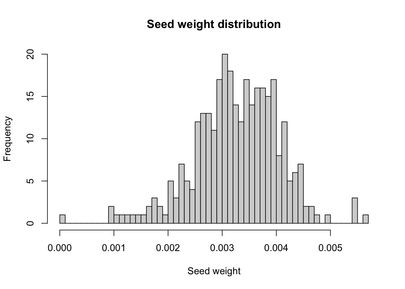
hist(traits$SeedWeight, main = "Seed weight distribution", 
        xlab = "Seed weight", breaks = 50)

Logic check: what does breaks actually do?

A histogram first bins the data — it cuts the value range into intervals (“bins”) and counts observations per bin. breaks is a suggestion for how many bins to use:

Default (~10 bins): the shape is blocky; broad features only.
breaks = 30: medium detail — real structure appears (this seed-weight distribution is right-skewed with a long thin tail).
breaks = 50: fine detail, but each bin holds fewer trees, so the counts get noisier and the shape gets jittery.

The trade-off is bias vs. variance: too few bins smooth over real features; too many bins amplify sampling noise. There is no single right answer — the point of the tabset is that you look at several and pick one that shows the structure without chasing noise. The x-axis is the variable’s value; the y-axis (default freq = TRUE) is the raw count per bin.

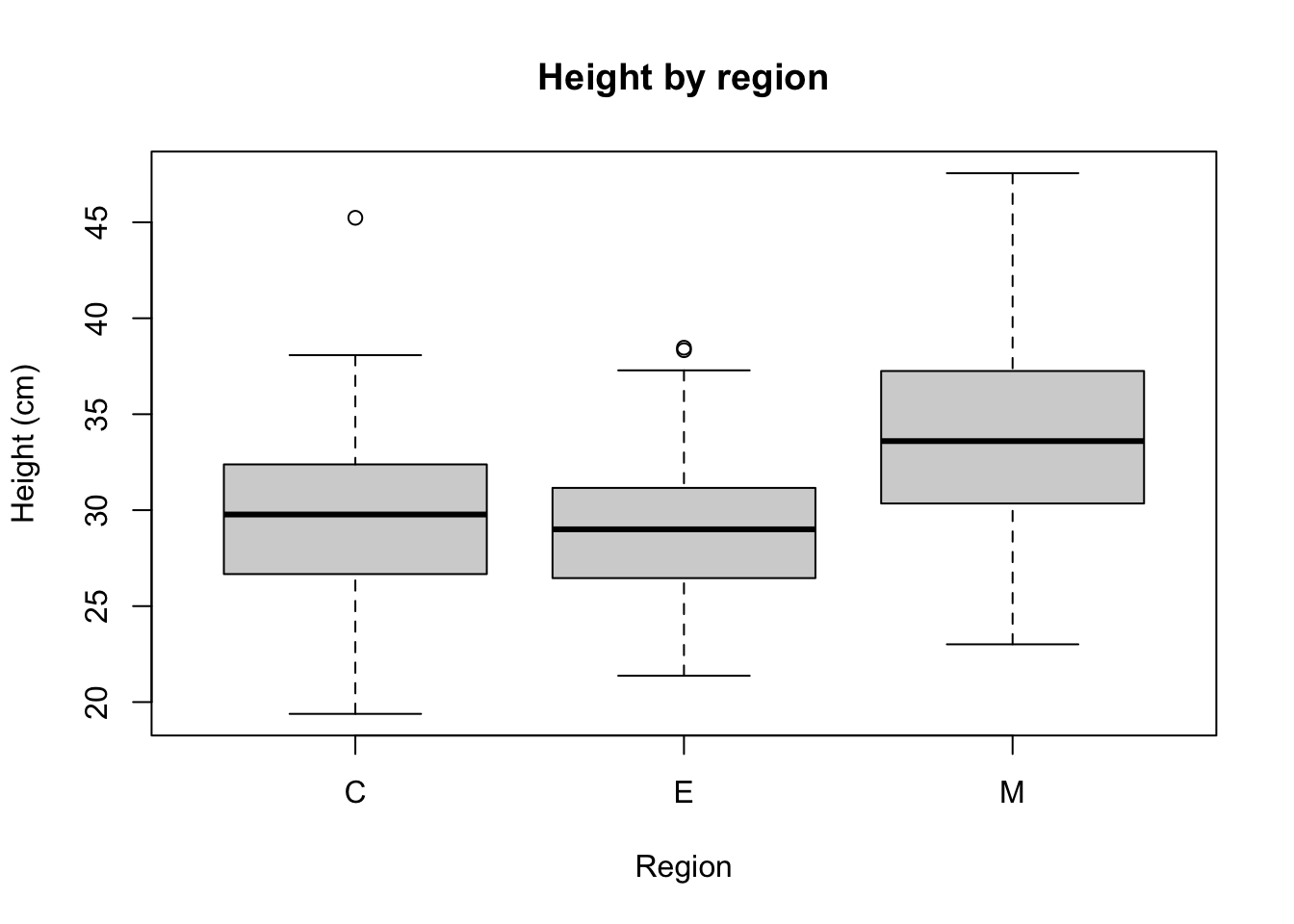
boxplot(Height ~ Region, data = traits, 
        main = "Height by region", 
        ylab = "Height (cm)")

Logic check: how to read this boxplot

For each region the box shows five numbers:

Bold center line — the median: C ≈ 29.8, E ≈ 29.0, M ≈ 33.6.
Box edges — the 1st and 3rd quartiles; the box spans the middle 50% of trees (the interquartile range, IQR).
Whiskers — the furthest values within 1.5 × IQR of the box.
Points beyond whiskers — individual outlier trees.

What the plot says: all three regions overlap heavily (heights between regions are not dramatically different), but region M sits visibly higher — its median exceeds the upper quartile of E. The medians differ even though the distributions overlap, which is precisely the situation where a comparison of groups (boxplot) is more informative than the overall histogram. Note summary() gives you these same five numbers numerically — the boxplot is summary() drawn.

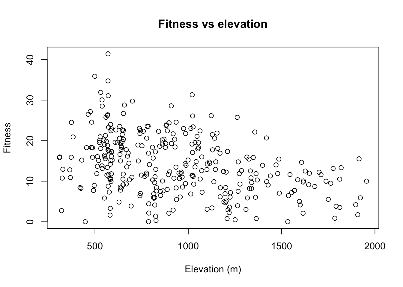
plot(traits$Elevation, traits$Fitness,
     xlab = "Elevation (m)", ylab = "Fitness",
     main = "Fitness vs elevation")

Logic check: reading a scatterplot

The cloud trends downhill: higher-elevation trees tend to have lower fitness. The correlation (computed in the exercises) is about −0.36 — a moderate negative association, not a tight line.

Two cautions before interpreting:

Association is not causation. Elevation here stands in for a whole bundle of correlated variables (temperature, growing season, soil). The plot cannot tell you which one matters.
Correlation ignores structure. The three regions occupy different elevation bands. A trend across regions might be a region effect (genetic origin) rather than an elevation effect — the confounding theme population genetics module tackles head-on with PCA before genotype–environment association.

Adding a fitted line summarizes the trend in one stroke:

plot(traits$Elevation, traits$Fitness,
     xlab = "Elevation (m)", ylab = "Fitness")
abline(lm(Fitness ~ Elevation, data = traits), col = "red", lwd = 2)

abline() draws a straight line from a model fit; lm() fits it. The col/lwd options style the line so it stands out from the points.

Saving outputs and scripting

pop_summary <- aggregate(cbind(Height, Fitness, SeedWeight) ~ Population, data = traits, FUN = mean)
write.csv(pop_summary, here::here("results/population_trait_summary.csv"), row.names = FALSE)

# exporting plot as a .png
png(here::here("results/height_by_region.png"), width = 800, height = 600)
boxplot(Height ~ Region, data = traits)
dev.off()

Code breakdown: the two save patterns

Tables. write.csv(x, file, row.names = FALSE) writes a data frame as CSV. row.names = FALSE suppresses the meaningless "1", "2", "3", ... column R would otherwise add — your data already has meaningful identifiers (Population).

Plots. Base R plots draw to a graphics device. By default that device is your screen; png() opens a file device instead, and everything you plot lands in the file until dev.off() closes it. The sequence is always:

png(path, width, height) — open the file device (dimensions in pixels)
draw: boxplot(...), hist(...), etc.
dev.off() — close the device and flush the file to disk

Forgetting dev.off() is the classic bug: the file stays empty, and every next plot you make goes into it instead of the screen. If plots stop appearing in your session, run dev.off() once and check results/.

Put everything into src/01_explore_traits.R and run it non-interactively — this is what makes it reproducible and Slurm-friendly:


Rscript src/01_explore_traits.R

Code breakdown: what makes a script “reproducible”?

A script (rather than typed commands) gives you three things:

A record — the exact sequence of steps, reviewable and citable.
Re-runnability — same script + same raw data = same outputs, on your laptop or on a Slurm node, forever. This is the working definition of reproducibility.
Scale — only a script can be handed to sbatch, scheduled overnight, or re-run when the data updates.

The skeleton to aim for in src/01_explore_traits.R:

# 01_explore_traits.R — first look at red spruce fitness traits
# Usage: Rscript src/01_explore_traits.R

# --- setup: paths (relative to project root) -----------------------------
raw_file <- here::here("data/raw/red_spruce_fitness_traits.txt")
out_dir  <- here::here("results")

# --- load ----------------------------------------------------------------
traits <- read.delim(raw_file, header = TRUE, sep = "\t",
                     stringsAsFactors = FALSE)

# --- inspect -------------------------------------------------------------
dim(traits)
str(traits)
colSums(is.na(traits))

# --- analyze -------------------------------------------------------------
pop_summary <- aggregate(cbind(Height, Fitness, SeedWeight) ~ Population,
                         data = traits, FUN = mean)

# --- save ----------------------------------------------------------------
write.csv(pop_summary, here::here(out_dir, "population_trait_summary.csv"),
          row.names = FALSE)

Notice the section comments — setup / load / inspect / analyze / save — and that not a single absolute path appears anywhere. Anyone can clone the project, run one command, and get your results.

Wrap up

Idea check

Answer these in your own words before moving to the exercises — write your answers as comments at the top of src/01_explore_traits.R.

What is the difference between a vector and a data frame in R?
Why prefer a relative path like "data/raw/red_spruce_fitness_traits.txt" over an absolute path like /home/your_username/...?
What does str(traits) tell you that head(traits) does not?
Why does treating Region as a factor (rather than plain character text) matter for boxplot(Height ~ Region, data = traits)?
If mean(traits$Height) returned NA, what would you check first, and how would you fix it?
Why write outputs into results/ instead of overwriting anything in data/raw/?

Sample answers

A vector is one-dimensional and holds a single type; a data frame is two-dimensional — a list of equal-length vectors, so each column can have its own type. Vectors are the building blocks; data frames organize them into one-observation-per-row tables.
Relative paths travel; absolute paths don’t. data/raw/... resolves correctly wherever the project lives — laptop, cluster, collaborator’s machine — while /home/your_username/... only exists on one computer. here::here() gives you relative-path portability even when the working directory is wrong.
str() reports the type of every column (chr/int/num) and the object’s shape — information about all 326 rows. head() only shows the first few rows’ values; a column mis-parsed as text looks identical in head() but announces itself in str().
A factor carries fixed, ordered levels, which the boxplot formula uses to define the groups and their axis order. Plain characters usually work here too, but factors give you control (alphabetical, or a biologically meaningful order), guarantee every category appears even with zero counts, and are what modeling functions like lm() expect for categorical predictors.
Check for missing values: sum(is.na(traits$Height)) — here, 13. Fix with mean(traits$Height, na.rm = TRUE). The deeper question — why are 13 heights missing and are they missing at random? — matters before you publish any number computed on the remaining 313.
data/raw/ is the immutable source: if analysis outputs overwrite it, you can no longer distinguish input from product, and re-running the script gives different (corrupted) results. Everything in results/ is disposable and regenerable from raw + script; the raw file is not.

Practical exercises

Work through these in order inside an R session, then consolidate the working code into src/01_explore_traits.R.

Exercise 1 — Load and confirm the shape

Load the dataset and confirm it has 326 rows and 19 columns.

Solution

traits <- read.delim(here::here("data/raw/red_spruce_fitness_traits.txt"),
                     header = TRUE, sep = "\t", stringsAsFactors = FALSE)
dim(traits)

[1] 326  19

dim() returns 326 19 — 326 trees, 19 variables. If you had gotten 327 rows, the likely culprit would be a header misread; 1 row, a wrong separator; and a single column, tabs not being recognized (check the actual file with head data/raw/red_spruce_fitness_traits.txt in the shell).

Exercise 2 — Map every column to its type

Run str(traits) and list every column name along with its type (chr, int, num).

Solution

str(traits) prints the full map. Grouped:

chr: Family, Population, Location, Region
int: Tree, Elevation
num: Latitude, Longitude, SeedWeight, Germination, Survival, Height, Fitness, PC1, PC2, Family_Homozygosity, Population_Homozygosity, Genetic_Diversity, Genetic_Load

That is 4 text, 2 integer, 13 numeric columns = 19 total. Sanity-check the biological plausibility of the types too: identifiers as text ✓, elevation in whole meters as integer ✓, proportions like Survival as numeric ✓. A type that surprises you (say, Height as chr) means some row contains non-numeric junk — find it with traits$Height[is.na(as.numeric(traits$Height))]-style checks.

Exercise 3 — Summary statistics, and the NA trap

Compute overall summary statistics (mean, sd, min, max) for Height and Fitness.

Solution

stats_of <- function(x) {
  c(mean = mean(x, na.rm = TRUE),
    sd   = sd(x, na.rm = TRUE),
    min  = min(x, na.rm = TRUE),
    max  = max(x, na.rm = TRUE))
}

rbind(Height  = stats_of(traits$Height),
      Fitness = stats_of(traits$Fitness))

            mean       sd      min      max
Height  30.03018 4.641802 19.38537 47.56003
Fitness 14.00769 7.320978  0.00000 41.42805

Expected values: Height mean 30.03, sd 4.64, range 19.39–47.56; Fitness mean 14.01, sd 7.32, range 0.00–41.43.

The critical detail: without na.rm = TRUE every one of these returns NA, because Height is missing for 13 trees and Fitness for 12. Writing your own stats_of() wrapper (a function — see the quick reference) bakes the na.rm in once instead of repeating it eight times. Note how rbind() stacks the two named rows into one table — the same row-binding idea you’ll meet again when combining populations in the population genetics module.

Exercise 4 — Count trees per group

Use table() to count trees per Population and per Region. Which population has the most trees sampled?

Solution

table(traits$Population)


   AB   ALB   APP   ASC     B   BAL   BBE   BER   BFA   BLA   BRA   BRB   BRU 
    4     5     6     6     5     6     5     6     5     5     5     4     5 
  CAM    CR   CRA   CRR    DG   EQU   ESC   G13   G18   G57   GPA   GRE    HR 
    6     5     6     2     5     6     6     5     3    11     4     6     5 
  HUN   IND   JAY   KAN   KIL   KOS   LEU   LOL   MAC   MMF   MPG   MRC   MSK 
    7     6     3     5     6     6     5     5     5     7     6     5     4 
   MT NBTIC   NOR   OCT   OKE   OWL   PRK   PRO    RP   SAV   SPR   TWI    WA 
    7     6     6     6     6     4     5     4     5     7     5     5     5 
  WCA   WHI   XBM   XCS   XCV   XDS   XFS   XGL   XPK   XSK   XWS 
    6     6     6     2     5     6     3     4     4     3     3

table(traits$Region)


  C   E   M 
178 101  47

which.max(table(traits$Population))

G57 
 23

table(traits$Region) → C: 178, E: 101, M: 47 — 178 + 101 + 47 = 326, so every tree has a region.
The most-sampled population is G57 with 11 trees; most populations have 4–7 trees, and a couple (CRR, XCS) have only 2.

which.max() returns the name of the maximum entry, automating the eyeball-scan. Keep the small populations in mind for Exercise 6 — means computed from 2 trees are far noisier than means from 11.

Exercise 5 — Subsetting with two conditions

Subset the data to trees in Region == "C" with Survival > 0.8. How many trees meet this criterion?

Solution

c_healthy <- traits[traits$Region == "C" & traits$Survival > 0.8, ]
nrow(c_healthy)

[1] 117

116 trees (out of 178 in region C). Points to notice:

The comma inside [ , ] is mandatory — without it you select columns matching a logical vector, a different (and here, nonsense) operation.
& combines the two conditions; both must hold for a row to survive.
One tree has NA for Survival, so its comparison is NA and the row is dropped silently — usually the right behavior, but be able to explain why.
Sanity check: nrow(c_healthy) = 116 ≤ 178 = table(traits$Region)["C"]. A filtered count larger than its parent group is impossible; catching that means your condition logic is broken (probably | where you meant &).

Exercise 6 — Grouped means

Use aggregate() or tapply() to get mean Height and mean Fitness per Population. Identify the top 3 populations by mean Fitness.

Solution

pop_means <- aggregate(cbind(Height, Fitness) ~ Population,
                       data = traits, FUN = mean)
head(pop_means[order(-pop_means$Fitness), ], 3)   # top 3 by Fitness

   Population   Height  Fitness
22        G18 33.12132 24.53187
13        BRU 40.61024 24.17780
11        BRA 32.56467 22.90860

tail(pop_means[order(-pop_means$Fitness), ], 2)   # bottom of the table, for contrast

   Population   Height  Fitness
62        XSK 26.40402 3.112958
63        XWS 30.18033 2.188637

Top 3 by mean fitness: G18 (24.53), BRU (24.18), BRA (22.91); the lowest are XWS (2.19) and XSK (3.11).

order(-pop_means$Fitness) sorts descending — the minus flips the order of an otherwise ascending sort. Read the results with the caveat from Exercise 4 in mind: G18 has only 3 trees, so its mean rests on a tiny sample; its rank could easily change with more sampling. Grouped means are only as trustworthy as the per-group counts behind them.

Exercise 7 — Plots, saved to files

Create a histogram of SeedWeight and a boxplot of Height by Region. Save both as PNG files in results/.

Solution

png(here::here("results/seedweight_hist.png"), width = 800, height = 600)
hist(traits$SeedWeight, breaks = 30,
     main = "Seed weight distribution", xlab = "Seed weight")
dev.off()

png(here::here("results/height_by_region.png"), width = 800, height = 600)
boxplot(Height ~ Region, data = traits,
        main = "Height by region", ylab = "Height (cm)")
dev.off()

The three-beat pattern each time: png() opens the file, the plot call draws into it, dev.off() closes and flushes. Verify the files exist afterwards with list.files(here::here("results")) — an empty file means you forgot dev.off(); plots appearing on screen instead mean png() never ran.

Exercise 8 — Save the summary table

Save your population-level summary table as results/population_trait_summary.csv.

Solution

write.csv(pop_summary,
          here::here("results/population_trait_summary.csv"),
          row.names = FALSE)

row.names = FALSE keeps the file keyed by Population alone — the CSV’s first column will be Population, not R’s meaningless 1, 2, 3, ... row numbers. Inspect it from the shell with head results/population_trait_summary.csv to confirm what your future self (and your collaborators) will actually receive.

Exercise 9 — The reproducibility test

Move all working code into src/01_explore_traits.R and confirm it runs cleanly end-to-end with Rscript src/01_explore_traits.R, producing the expected files in results/.

Solution sketch

The pass/fail test is a clean-room re-run:

# from the project root
rm -rf results                # delete everything R ever produced
Rscript src/01_explore_traits.R
ls -lh results/                # the script must recreate it all

If that sequence recreates population_trait_summary.csv plus the two PNGs with no errors and no warnings you can’t explain, your module is reproducible. If it fails, the usual culprits are, in order: a hard-coded absolute path, a missing dir.create(results) before the first write, and code that depends on objects you created interactively but never put in the script. The last one is the reason to build scripts from a fresh R session, not from the session where you explored.

Homework

Compute summary statistics (mean, sd, min, max) for at least 4 traits (e.g., Height, Fitness, SeedWeight, Germination), broken down by both Population and Region.
Produce at least 3 plots: one histogram, one boxplot grouped by Region, and one scatterplot relating two continuous variables (e.g., Elevation vs. Fitness). Save all three to results/.
Write your interpretation as comments at the bottom of the script, answering:
- Which population has the highest and lowest mean fitness?
- Is there a visible relationship between elevation and fitness or seed weight? Describe it in one or two sentences.
Bonus (optional): recreate one plot with ggplot2 instead of base R.

Hints (not full answers)

Grouped by Region first — it’s only 3 groups, so eyeball-able: mean Height is C 29.7 / E 28.9 / M 34.0 and mean Fitness C 14.7 / E 10.6 / M 19.8. Region M — the group with the lowest median elevation (570 m, vs. 787 for C and 1333 for E) — is taller and higher-fitness on average. Per-population, extend the aggregate(... ~ Population) pattern from Exercise 6; for two grouping factors at once, try aggregate(cbind(...) ~ Region, ...) separately — a Population × Region cross needs table(traits$Population, traits$Region) or interaction().
The scatterplot answer you should arrive at: elevation vs. fitness is a moderate negative relationship (correlation ≈ −0.36) — higher sites, lower mean fitness; elevation vs. seed weight is weakly positive (≈ +0.25). Both are visible-but-loose trends in the point cloud, not tight lines. Remember the two cautions from the plotting section before you write the interpretation: association ≠ causation, and region structure is confounded with elevation here.
ggplot2 bonus: the same boxplot is ggplot(traits, aes(x = Region, y = Height)) + geom_boxplot() after install.packages("ggplot2") and library(ggplot2) — the + layers replace the single-call-with-arguments style of base plotting.

Goal

Prerequisites

Learning objectives

R quick reference

Setting up your R project

R data types and structures

The four structures, one at a time

Missing values: NA, the silent saboteur

Importing and inspecting the dataset

Indexing and subsetting

How the bracket syntax works

Summarizing data

What each summarizer is for

Basic plotting

Saving outputs and scripting

Wrap up

Idea check

Practical exercises

Exercise 1 — Load and confirm the shape

Exercise 2 — Map every column to its type

Exercise 3 — Summary statistics, and the NA trap

Exercise 4 — Count trees per group

Exercise 5 — Subsetting with two conditions

Exercise 6 — Grouped means

Exercise 7 — Plots, saved to files

Exercise 8 — Save the summary table

Exercise 9 — The reproducibility test

Homework

Missing values: `NA`, the silent saboteur